Solid Mechanics
Now it is time to define the physics settings, such as material models, loads, and constraints. Initially, the analysis was specified to be stationary, using the classical equations associated with solid mechanics.
By default, the Solid Mechanics interface assumes that the participating material models are linear elastic, which is appropriate for this example.
Fixed Constraint 1
Assume that the boundaries of the bolt holes are perfectly constrained.
1
2
3
Boundary Load 1
The load acts radially outward in the holes. There are several ways in which you can achieve that. You can, as shown here, use the cylindrical coordinate system. Alternatively, you could have used the built-in Boundary System, or you could simply have applied it as a pressure load.
1
2
3
4
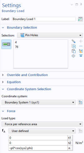
In the n-component text field, type -p0*cos(sys2.phi). The normal direction in a boundary system points outward from the surface, hence the negative sign in front of the pressure load.
5
6
The settings you have made for the frames in the two coordinates systems do not have any effect in the current model, since the analysis will assume geometric nonlinearity. If, however, the model is extended later to include effects of geometrical nonlinearity, then the choice of frames in various features will matter. Similarly, it does not matter here whether you choose Force per reference area or Force per deformed area as long as the analysis is geometrically linear.
There are several different ways in which this load could have been described without making use of a position dependence when defining the coordinate system. You could, for example, use two separate Boundary load nodes with different signs in front of the load. Alternatively, you could still use a single Boundary load node, but with the expression p0*abs(cos(sys2.phi)) or p0*cos(sys2.phi)*sign(X)