The Hydrodynamic Bearing (hdb) interface (

), found under the
Structural Mechanics >
Rotordynamics branch (

) when adding a physics interface, is intended for analysis of fluid-film bearings in 3D, modeled using a surface geometry. It is assumed that the thickness of the film is very small. Different types of journal bearings, such as cylindrical, elliptical, split halves, multilobe, and tilting pad bearings, can be modeled using the
Hydrodynamic Journal Bearing feature in this interface. You can also model a bearing mounted on a foundation.
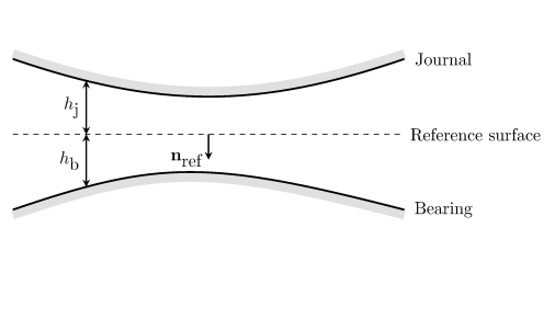
Using equations on the reference surface, the Hydrodynamic Bearing interface computes the pressure in a narrow gap between the journal and the bearing. When modeling the flow, it is assumed that the total gap height, h = hj + hb, is much smaller than the typical lateral dimension
L of the reference surface. This physics interface is used to model laminar flow in thin gaps or channels in, for example, a lubricating oil between two rotating cylinders.
The Hydrodynamic Journal Bearing node is always added, with the
Cylindrical bearing as the default. This node adds the Reynolds equations for the pressure distribution on the film surface and has a Settings window to define the bearing properties. The equations in this feature also account for the velocity due to the axial rotation of the rotor.
When the Hydrodynamic Bearing interface is added, these default nodes are also added to the
Model Builder —
Bearing Orientation (the orientation of the bearing in the spatial frame),
Border (a boundary condition where lubricant is assumed to flow out into a space filled with the same fluid), and
Initial Values. Then, from the
Physics toolbar, you can add features that implement other boundary conditions and bearing properties. You can also right-click
Hydrodynamic Bearing to select physics features from the context menu.
The Label is the default physics interface name.
The Name is used primarily as a scope prefix for variables defined by the physics interface. Refer to such physics interface variables in expressions using the pattern
<name>.<variable_name>. In order to distinguish between variables belonging to different physics interfaces, the
name string must be unique. Only letters, numbers, and underscores (_) are permitted in the
Name field. The first character must be a letter.
The default Name (for the first physics interface in the model) is
hdb.
For Liquid with cavitation enter the
Cavitation transition width (SI unit: Pa). The default is 1 MPa.
Select the Calculate dynamic coefficients checkbox to enable computation of the equivalent stiffness and the damping coefficients for the bearing.
To display this section, click the Show More Options button (

) and select
Stabilization in the
Show More Options dialog. This section is only available when
Liquid with cavitation is selected in the
Physical Model section.
Select the Isotropic diffusion checkbox to include the stabilization of the Reynolds equation with cavitation and then enter a
Tuning parameter value. A larger value of the tuning parameter increases the amount of isotropic diffusion in the system.
Enter a Reference pressure level pref. The default value is
1[atm]. This pressure represents the ambient pressure, which is not accounted for when computing fluid loads.
Select the Pressure discretization —
Linear,
Quadratic,
Cubic, or
Quartic to change the order of the shape functions for the pressure.
The dependent variable (field variable) is the Pressure pf. The name can be changed but the names of fields and dependent variables must be unique within a component.