The Navier–Stokes equations can be nondimensionalized for a domain whose width (h0) is much smaller than its lateral dimension(s) (l0) (see Ref. 1 for a detailed discussion). When Re(h0/l0)2 << 1, and terms of order (h0/l0)2 and higher are neglected, the Navier–Stokes equations reduce to a modified form of the Stokes equation, which must be considered in conjunction with the continuity relation.

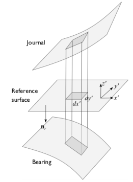
The equations are most conveniently expressed in a local coordinate system in which x' and y' are tangent to the plane of the reference surface, and z' is perpendicular to the surface, as illustrated in Figure 7-4. Using this coordinate system

Here pf is the pressure resulting from the fluid flow, μ is the fluid viscosity, and (vx', vy') is the fluid velocity in the reference plane (which varies in the z' direction).

The constants C1x', C2x', C1y', and C2y' are determined by the boundary conditions.

Equation 7-4 shows that the flow is a linear combination of laminar Poiseuille and Couette flows. The velocity profile is quadratic in form, as shown in Equation 7-5.

The average flow rate in the reference plane, vav, is given by

The forces acting on the journal are determined by the normal component of the viscous stress tensor, τ, at the journal and bearing walls (τn, where n is the normal that points out of the fluid domain). The viscous stress tensor takes the form

Neglecting the gradient terms, which are of order h0/l0, results in the simplified stress tensor

The components of the stress tensor can be expressed in terms of the velocity and pressure gradients using Equation 7-4. Note that the normals to both the journal and the bearing are parallel to the z' direction, to zeroth order in h0/l0. The forces acting on the bearing and the journal are therefore given by

Assuming a slip length of Lsj at the journal, and a slip length of Lsb at the bearing, the general slip boundary conditions are given by:

For nonidentical slip lengths, the constants C1x', C2x', C1y', and C2y' take the following values:

where vav,c is a term associated with Couette flow, and vav,p is a coefficient associated with Poiseuille flow (see Table 7-1 below).

Note that the z' direction corresponds to the −nr direction. The x' and y' directions correspond to the two tangent vectors in the plane. Using vector notation, the forces become:

In Equation 7-8 it is assumed that nj = −nr and nb = nr. In COMSOL Multiphysics the accuracy of the force terms is improved slightly over the usual approximation (which neglects the slope of the journal and bearing as it is of order h0/l0) by using the following equations for nj and nb:

These definitions are derived from Equation 7-4 and Equation 7-5 and include the additional area that the pressure acts on as a result of the slopes of journal and bearing surfaces.

where fj,p is the Poiseuille coefficient for the force on the journal, and fj,c incorporates the Couette and normal forces (due to the pressure) on the journal. Similarly, fb,p is the Poiseuille coefficient for the force on the bearing, and fb,c incorporates the Couette and normal forces (due to the pressure) on the bearing.

The cases of identical slip length and no slip are limiting cases of the formulas derived above. The main results are summarized in Table 7-1, where the constants defined in Equation 7-7 and Equation 7-9 are used.