The Label is the physics interface name. The default is Geometrical Optics.

The Name is used primarily as a scope prefix for variables defined by the physics interface. Refer to such physics interface variables in expressions using the pattern <name>.<variable_name>. In order to distinguish between variables belonging to different physics interfaces, the name string must be unique. Only letters, numbers, and underscores (_) are permitted in the Name field. The first character must be a letter.

The default Name (for the first physics interface in the model) is gop.

Select an option from the Wavelength distribution of released rays list: Monochromatic (the default), Polychromatic, specify vacuum wavelength, or Polychromatic, specify frequency.

The Maximum number of secondary rays limits the total number of secondary rays that can be created by capping them at the specified number. Secondary rays are released when an existing ray is subjected to certain boundary conditions. For example, when a ray arrives at a Material Discontinuity or Scattering Boundary between different media, the incident ray is refracted and a reflected ray is created; the degrees of freedom for this reflected ray are taken from one of the available secondary rays, which are preallocated when the study begins. Secondary rays are also used to model the interaction of rays with diffraction gratings, using the Grating boundary condition.

If an insufficient number of secondary rays are preallocated, a reflected ray may not be released when an existing ray undergoes refraction, even if some radiation should be reflected at the material discontinuity, and a warning message will be generated by the study. However, if a very large number of secondary rays are preallocated, then the number of degrees of freedom may become unnecessarily large. Thus, the Maximum number of secondary rays should only be large enough that all reflected rays which significantly affect the solution can be released. Rays that undergo total internal reflection at material discontinuities are not considered secondary rays and do not require extra preallocated degrees of freedom.

By default, the Use geometry normals for ray-boundary interactions checkbox is checked. In this case, the surface normal is computed from an analytic representation of the geometry surfaces, if such a representation can be obtained. If this checkbox is cleared, the surface normal is computed using the underlying mesh discretization of the boundary rather than the exact shape of the geometry itself.

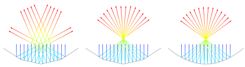
For the simple case of ray reflection by a parabolic edge in 2D, three example plots are shown in Figure 3-1 below. In the leftmost plot, linear geometry shape order has been specified; in other words, Linear has been selected from the Geometry shape order list in the settings for the model component. The left figure also uses mesh normals. The reflected ray directions are visibly inaccurate because the boundary mesh is very coarse. The center figure uses Linear geometry shape order and geometry normals. Although the mesh is equally coarse, the reflected ray directions are much more accurate. The rightmost figure uses Quadratic shape order; because the edge is parabolic, this shape order results in reflected ray directions that are exact (to within machine precision) no matter whether mesh normals or geometry normals are used, because quadratic elements can perfectly represent a parabola.

The Use geometry normals for ray-boundary interactions checkbox has no effect on the solution if the mesh can deform. This is true, for example, when the geometry is subjected to structural loads or thermal stresses. Then the mesh normal is always used.

By default the Only store accumulated variables in solution checkbox is cleared. If this checkbox is selected, then the degrees of freedom associated with individual rays (such as the ray position, wave vector, intensity, power, and normalized Stokes parameters) will be solved for but not stored in the solution data. However, certain physics features define degrees of freedom in domains or on boundaries rather than on the individual rays, and these degrees of freedom will be retained in the solution. These quantities, called accumulated variables, are defined by the following features:

While the Only store accumulated variables in solution checkbox is selected, if you run a study for the first time, the default Ray dataset and Ray Trajectories plot will not be created. If you later clear the checkbox and recompute the study, you may need to add these Results features manually.

Use this section to control the properties of the void exterior to the model geometry as well as the properties of domains outside of the selection of the Geometrical Optics interface. For further details about what constitutes a “void” region, see the Geometry and Meshing section of the Ray Optics Modeling chapter.

Select an option from the Optical dispersion model list: Absolute vacuum, Specify refractive index (the default), or Air, Edlén (1953). This setting controls the refractive index in the empty space outside the geometry, called the void region. It also controls the refractive index for domains that are not included in the selection of the Geometrical Optics interface.

For any type of optical dispersion model in the exterior and unmeshed domains, the algorithm to trace rays assumes that the medium is homogeneous. If a graded-index material is present, then its domain should be included in the selection of the Geometrical Optics interface and the spatial dependence of the refractive index should be controlled from the Medium Properties node.

Select an option from the Intensity computation list: None (the default), Compute intensity, Compute power, Compute intensity and power, Compute intensity in graded media, or Compute intensity and power in graded media. For None no additional variables are computed along the rays. For other options, the ray intensity or ray power is computed as described below.

The Compute phase checkbox is only shown if the ray intensity is computed. Select the checkbox to allocate an auxiliary dependent variable for the phase of each ray. When the phase of each ray is computed, it is possible to plot interference patterns and visualize the instantaneous electric field components of polarized rays in postprocessing. When this checkbox is selected, the total number of degrees of freedom increases by 1 per ray. This option is based on the assumption that the coherence length of the radiation is arbitrarily large.

The Use corrections for strongly absorbing media checkbox is shown if the ray intensity is computed. Select the checkbox to accurately model reflection and refraction of rays at boundaries between strongly absorbing media, in which the imaginary part of the refractive index is very large. This option allocates two or three auxiliary dependent variables per ray based on space dimension. For more information about the way this option affects the intensity calculation, see Refraction in Strongly Absorbing Media in Theory for the Geometrical Optics Interface.

When the Intensity computation is set to Compute intensity in graded media or Compute intensity and power in graded media enter a Tolerance for curvature tensor computation (dimensionless). This tolerance is used internally when computing the principal radii of curvature of propagating wavefronts in a graded medium. A larger tolerance makes the solution less accurate but more stable.

Additionally, when the ray is released inside a medium with a complex and spatially dependent refractive index (that is, a graded and lossy medium), you must select Release inside graded and dissipative medium checkbox in the corresponding release feature. The checkbox appears when

Select the Compute optical path length checkbox to allocate an auxiliary dependent variable for the optical path length of each ray. The default variable name is gop.L. It is possible to reset the optical path length to 0 when rays interact with boundaries.

Select the Count reflections checkbox to allocate an auxiliary dependent variable for the number of reflections undergone by each ray, including reflections by the Wall and Material Discontinuity features. The default variable name is gop.Nrefl. The auxiliary variable begins at 0 when rays are released and is incremented by 1 every time a ray is reflected at a boundary.

Select the Store ray status data checkbox to add new variables for quantities that cannot necessarily be recovered from the ray trajectory data alone. This is especially true if automatic remeshing is used in a model. The variables created include the following, all of which would be preceded by the physics interface tag (for example, gop.):

The global variable names in Table 3-1 all take the unreleased secondary rays into account. For example, suppose an instance of the Geometrical Optics interface includes 100 primary rays and 100 allocated secondary rays. At the last time step, suppose that 80 of the primary rays have disappeared at boundaries and that 40 secondary rays have been emitted, all of which are still active. Then the variable gop.fac, the fraction of active rays at the final time step, would have the value (20 + 40)/(100 + 100) or 0.3.

Select an option from the Results list: None (the default), Plot spot diagram, or Plot spot diagram and geometric MTF. For None, only the Ray trajectories plot is created. For other options, the default plots are set up as follows:

The datasets created have the unique tag of the preceding data source in the label. For example, an Evaluation Group that uses data from a Release from Grid has the label LSF Data (relg1), where relg1 is the unique tag of the Release from Grid feature. Subsequently, the Kernel Density Estimation (KDE) datasets generated from such an Evaluation Group have the labels LSFx (eg1) or LSFy (eg1) for the x and y coordinates of the Intersection Point 3D dataset space variables, where eg1 is the unique tag of the Evaluation Group feature. These naming conventions are propagated to the Spatial FFT datasets, the Line Graph plots, and their legends.

The Plot MTF in single plot group checkbox is only shown if Plot spot diagram and geometric MTF is selected. If it is checked (default), then MTF for all release features are plotted in the same plot group. Otherwise, a new plot group is created for every release feature.

This section is only shown when Advanced Physics Options are enabled (click the Show More Options button  in the Model Builder toolbar, and select Advanced Physics Options in the Show More Options dialog). These options are hidden by default because it is only necessary to modify them under very specific circumstances.

The Wall accuracy order sets the accuracy order of the time stepping used for time steps during which a ray-wall interaction happens. Select an order of 1 to use a forward Euler step and compute the direction or ray propagation both before and after the wall interaction. Select an order of 2 (the default) to use a second-order Taylor method to compute the trajectory before the wall interaction. After the ray-wall interaction a second-order Runge–Kutta method is used. Usually this setting has no effect on the ray tracing calculation because the rays move along straight lines, but the higher wall accuracy order is more accurate if graded-index media are present.

Select an option from the Arguments for random number generation list: Generate unique arguments (the default), Generate random arguments, or User defined. This setting determines the behavior of the different random number generators (RNGs) used in the Ray Optics Module.

Certain features such as the Wall boundary condition with the Diffuse scattering wall condition utilize the random and randomnormal functions to generate random numbers. Typically the random numbers are functions of the ray index, time, a unique input argument for different variable definitions, and another argument i, which is controlled by this setting.

The effect of the three options on the additional argument i and the seed are described below:

Note that the random function is a pseudorandom number generator (PRNG), not a true random number generator (RNG) in the sense that an observer with perfect knowledge of the algorithm and a history of previously generated values could predict the ensuing values. However, PRNG is sufficient for most purposes.

The Allow multiple release times checkbox, which is cleared by default, allows an array of release times for the rays to be specified in any of the ray release features. If the checkbox is cleared, all rays are released at time t = 0.

By default the Exclude Jacobian contributions from ray equations checkbox is cleared. If this checkbox is selected, then expressions for the time derivatives of the degrees of freedom on rays are not included in the Jacobian matrix. Excluding contributions to the Jacobian can significantly improve solution time if the number of rays in the model is very large. The drawback is that the Jacobian is not exact, so smaller time steps or path length intervals may be needed to obtain an accurate solution. This drawback is most noticeable when computing the ray intensity or power in an absorbing medium.

By default the Treat unmeshed releasing entities as errors checkbox is selected. Certain ray release features, such as the Release and Release from Boundary features, compute the ray release positions based on a geometric entity, which must be meshed. While this checkbox is selected, failure to mesh the selections of such features will result in an error message when running any study in the model. If this checkbox is cleared, failure to mesh the selections of such features will result in them releasing zero rays, but will otherwise not interrupt the computation. Other physics features will still be able to release rays normally.

Enter a value for the Maximum number of wall interactions per time step. The default value is 1000. If a ray undergoes more than the specified number of boundary interactions in a single time step taken by the solver, the ray will disappear. This is included as a safeguard to prevent rays from getting stuck in infinite loops if the time between successive ray-wall interactions becomes infinitesimally small.

The dependent variables (field variables) are the components of the Ray position and Wave vector. The name can be changed but the names of fields and dependent variables must be unique within a model. In 3D, the default ray position vector components are qx, qy, and qz; and the default wave vector components are kx, ky, and kz.