Results
Running the study causes the following default nodes to appear under Results :
-
-
Ray Diagrams
In the following steps, two different ray diagrams are created, one of which uses a custom color expression. Begin by making some modifications to the default Ray Trajectories plot.
Cut Plane 1
1
Ray Trajectories
1
2
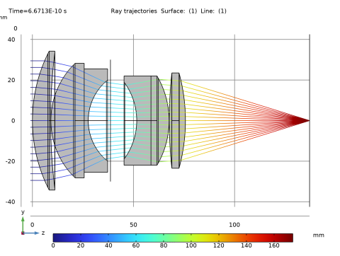
In the Settings window for 3D Plot Group, type Ray Diagram 1 in the Label text field.
3
4
Filter 1
5
6
7
In the Logical expression for inclusion text field, type at(0,abs(gop.deltaqx)<0.1[mm]). This logical expression will render rays in the yz-plane. In this expression, at() is a special operator that takes two arguments. It evaluates the second argument at the solution time given by the first argument, so the logical expression abs(gop.deltaqx)<0.1[mm] is being evaluated at the initial ray positions.
The variable gop.deltaqx is the x-component of the displacement of each individual ray relative to the average position of all rays.
In the following steps, the cross-section of the lens is rendered.
Surface 1
1
2
3
4
Line 1
1
2
3
4
5
Ray Diagram 2
For the second ray diagram rays will be colored according to the radial distance from the ray’s location in the image plane to the centroid. This makes it possible to visualize which rays are contributing to the image plane spot aberrations.
1
2
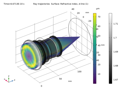
In the Settings window for 3D Plot Group, type Ray Diagram 2 in the Label text field.
3
4
5
Ray Trajectories 1
In the Ray Diagram 2 toolbar, click More Plots and choose Ray Trajectories .
Color Expression 1
1
2
In the settings for Color Expression 1 , locate the Expression section. In the Expression text field, type at(‘last’,gop.rrel). This is the radial coordinate relative to the average ray position in the image plane.
3
4
Surface 1
1
2
3
Selection 1
1
2
3
Transparency 1
1
2
3
4
Spot Diagram
In the following steps, a spot diagram is created.
2D Plot Group 3
1
2
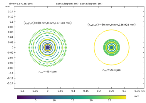
In the Settings window for 2D Plot Group, type Spot Diagram in the Label text field.
3
4
Spot Diagram 1
1
2
3
4
Color Expression 1
1
2
Locate the Expression section. In the Expression text field, type at(0,gop.rrel). This is the radial coordinate relative to the centroid at the location of the ray release. This allows the origin of each ray to be visualized.
3
The first spot diagram shows the intersection of the rays with the nominal image plane. This surface has been positioned so as to give the best image quality over a large range of field angles when using polychromatic light. A second spot diagram can be generated automatically on the plane which minimizes the RMS image quality for a selected field angle and wavelength.
Spot Diagram 2
1
2
3
4
Note: If the best focus plane lies behind the image plane, then the Freeze condition on the Wall defining the Image surface should be disabled. Currently the Intersection Point dataset can only compute real intersections of rays with the plane, not intersections of extrapolated ray positions.
5
6
7
8
The double Gauss lens spot diagram. On the left is the spot on the nominal image surface. The spot on the right is located at the “best focus” image plane that has been computed automatically.
Optical Aberration Diagram
In the following steps, an optical aberration diagram is created.
2D Plot Group 4
1
2
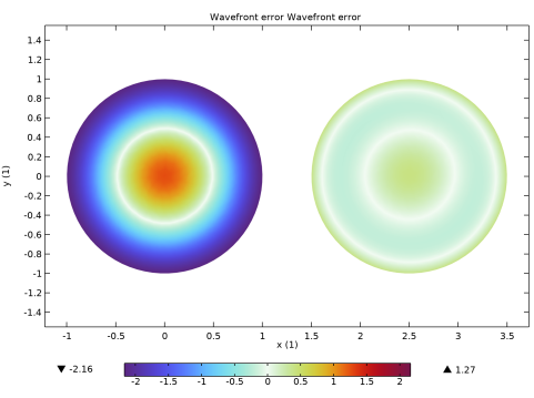
In the Settings window for 2D Plot Group, type Optical Aberration Diagram in the Label text field.
3
4
Optical Aberration 1
1
2
3
4
5
The advantage of using the Dipole color table with a symmetric color scale is that positive wavefront error will be shown in shades of red whereas negative wavefront error will be shown in blue. Bands of white indicate regions where the wavefront error is zero.
Optical Aberration 2
1
2
3
4
5
6
7
8
9
The double Gauss lens optical aberration diagram. The plot on the left uses all Zernike terms. In the plot on the right, the piston and defocus terms have been removed. Spherical aberration dominates the remaining terms.