|
1
|
|
3
|
In the Vacuum wavelength text field, type lambda. This wavelength was defined in the Parameters node.
|
|
4
|
Locate the input for the Center location (qc) vector. For the x, y, and z components, type dx, dy, and dz, respectively. These global parameters are defined in the Parameters 2: General
|
|
5
|
Locate the input for the Cylinder axis direction (rc) vector. For the x, y, and z components, type nix, niy, and niz, respectively.
|
|
6
|
|
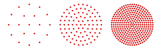
7
|
In the number of radial positions (Nc) text field, type N_ring, a global parameter with a value of 18. Below the text field, the Settings window will report that the hexapolar grid contains a total of 1027 grid points.
|
|
8
|
Locate the Ray Direction Vector section. For the x, y, and z components of the Ray direction vector (L0), type vx, vy, and vz., respectively.
|
|
2
|
In the Settings window for Wall, type Obstructions in the Label text field.
|
|
2
|
In the Settings window for Wall, type Stop in the Label text field.
|
|
2
|
In the Settings window for Wall, type Image in the Label text field.
|