Modeling Tools
In addition to the physics features described previously, the Ray Optics Module provides a variety of tools to help you set up your model and analyze results.
Optical Material Library
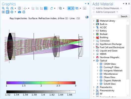
The Optical Material Library features more than 1700 materials, including more than 500 optical glasses. For most of these glasses, the refractive index is defined using optical dispersion coefficients to support accurate ray tracing of polychromatic light. Many of these glasses also include tabulated internal transmittance data as a function of wavelength, enabling volumetric light absorption to be predicted, as well as coefficients that describe the temperature dependence of the refractive index. Finally, most optical glasses include additional properties such as density, Young’s modulus, Poisson’s ratio, thermal conductivity, specific heat capacity, and thermal expansion coefficient, which facilitate coupled structural-thermal-optical performance (STOP) analysis.
The Optical Material Database (right) and the wavelength-dependent refractive index of a typical entry (left). The grayscale surface plot shows the d-line refractive index. Rays of three field angles are shown.
Part Library
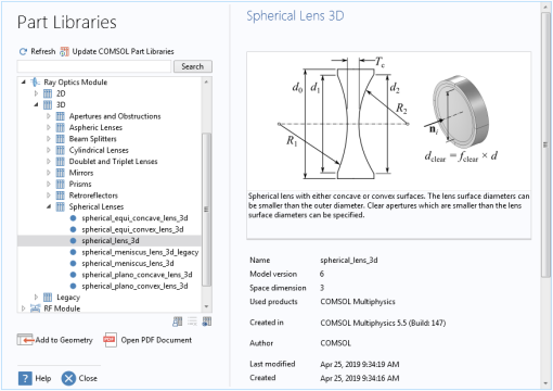
The Ray Optics Module includes a dedicated Part Library. This Part Library contains geometric entities that are frequently used in Ray Optics simulations. This includes spherical and aspheric lenses and mirrors, as well as retroreflectors, prisms, aperture stops, and beam splitters. These geometry parts are fully parameterized and include a variety of predefined selections that allow, for example, anti-reflective coatings to be applied to the exterior surfaces of a large number of lenses with ease.
The Part Library for the Ray Optics Module.
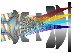
The compact camera module model uses spherical and aspheric lenses from the Part Library.
Ray Sources
The Geometrical Optics interface provides a variety of ray sources, called ray
release features
, to specify the initial position and direction of rays. Any number of ray sources of different types can be used in the same model.
Grid Sources
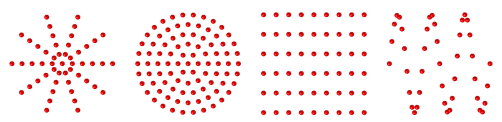
The most direct way to specify the ray release positions is with a grid-based release. As shown below, there are several ways to control the initial positions of the rays.
At each release position, the rays can propagate outward in a single direction or in a spherical, hemispherical, conical, or Lambertian (cosine law) distribution. A dedicated Solar Radiation feature is also available to initialize the ray direction based on the location on Earth’s surface and the date and time.
Rays can be released in a cylindrical (far left), hexapolar (middle left), rectangular (middle right), or nonuniform grid (far right).
Domain and Boundary Sources
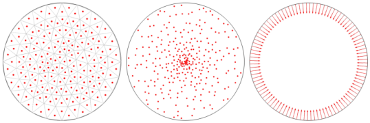
You can release rays from a selected set of domains or boundaries. The distribution of release points can be uniform, proportional to a user-defined density function, random, or based on the underlying finite element mesh.
Release positions based on the domain mesh (left), nonuniform density expression (middle), and uniformly distributed along a boundary (right).
Illuminated Surfaces
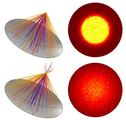
If you know that light will be reflected or refracted by a surface somewhere in the model geometry, you do not need to explicitly model the path of the incident light. Using the Illuminated Surface node, you can release reflected or refracted light directly from the selected boundary, just by specifying the direction of the incident light that hits it. There is also a built-in option to release reflected or refracted sunlight. Optionally, perturbations due to surface roughness and the solar limb darkening effect can be included.
Note that the Illuminated Surface node does not consider shading of the selected boundary; it assumes that the entire surface can release reflected or refracted light. If part of the surface is obscured or vignetted, it is still necessary to trace the incident rays on their path toward the surface.
Rays released from an illuminated solar reflector and resulting concentration ratios in the focal plane. The top row is the ideal case. The bottom row includes surface roughness and solar limb darkening effects.
Gaussian Beams
While solving for ray intensity or power, you can use the Gaussian Beam ray release feature to launch rays with a Gaussian intensity or power distribution.
The Geometrical Optics interface can only make rays follow curved paths if the medium has a graded refractive index. Rays do not behave exactly like a Gaussian beam in the vicinity of a beam waist, where the curvature of isosurfaces of constant phase can change nonlinearly as a function of distance along the nominal beam axis. Therefore, the Gaussian Beam ray release feature is only appropriate to use in the asymptotic limits where the geometry is either much larger or much smaller than the Rayleigh range.
Release of a Gaussian beam from a point. The ray power is a Gaussian function of the release angle. This type of power distribution is appropriate when the geometry is much larger than the Rayleigh range.
Blackbody Radiation
You can use the Blackbody Radiation node to release rays from a surface based on the temperature. The total power of the released rays follows the Stefan–Boltzmann law, the distribution of released ray directions is diffuse with respect to the surface normal, and the distribution of wavelength or frequency (for polychromatic ray releases) follows Planck’s law.
Other Sources
Rays can be released from selected points in a geometry. In 3D, they can also be released in selected edges. Thus, rays can be released from geometric entities of any dimension, up to the full dimension of the model.
It is also possible to load the release positions and initial directions from a text file, where each column provides one of the position or direction vector components. The distribution of loaded ray positions can undergo dilation, translation, rotation, or any combination of these three transformation types.
While solving for the intensity along rays, you can also import photometric data files to control the intensity distribution of the released rays.
Ray-Thermal Coupling
If the refractive indices in a ray optics model are complex-valued, then the imaginary part is treated as an absorption term. A ray propagating through a complex-valued refractive index loses some of its energy through this attenuation, and it is possible to deposit an equal amount of energy into the surrounding domain as a heat source term.
A dedicated Multiphysics interface, the Ray Heating interface, is available to use the heat generated by ray propagation in absorbing media with another physics interface for computing temperature, such as the Heat Transfer in Solids interface. The Ray Heating interface enables bidirectional couplings to be set up, allowing phenomena such as thermal lensing to be modeled.
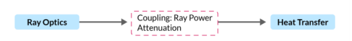
Unidirectional coupling from ray optics to heat transfer.
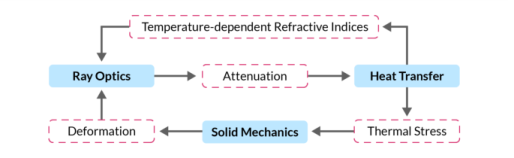
Bidirectional coupling between ray optics and heat transfer, including thermal stress.
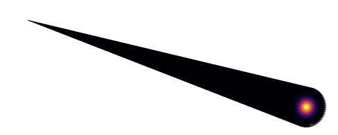
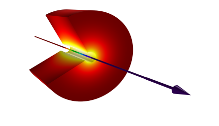
A ray passes through a layer of absorbing material, causing the temperature in the layer to increase.
Multiscale Electromagnetics Modeling
The Geometrical Optics interface uses the assumption that the wavefronts represented by rays are locally plane. Thus, the rays should be far away from any objects that are comparable in size to the wavelength. Diffraction effects are also ignored. In other words, ray tracing requires an
optically large
modeling domain.
Other optional add-on modules for COMSOL Multiphysics provide physics interfaces that solve Maxwell’s equations in the frequency domain, allowing accurate calculation of the fields in a wavelength-scale geometry. These interfaces can fully resolve every oscillation of the electric field with a finite element mesh, but they become computationally expensive if the geometry spans a large number of wavelengths. For second-order elements, about 5 elements per wavelength are needed (the
Nyquist criterion
).
For true multiscale modeling of electromagnetic wave propagation, in which a wavelength-scale source releases radiation into an optically larger geometry, a combination of numerical methods is needed. The Geometrical Optics interface includes features that use the results of a frequency domain electromagnetics model to define a ray source, such as the Release from Electric field node and the Release from Far-Field Radiation Pattern node.
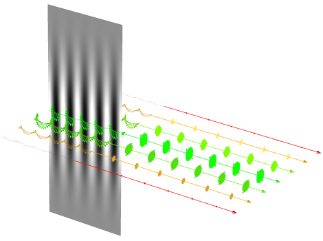
The propagation of a Gaussian beam is modeled using the Electromagnetic Waves, Beam Envelopes interface. Then rays are released from the adjacent surface. The rays are assigned their initial intensity and polarization based on the tangential electric field. Polarization ellipses are drawn along the rays.
Releasing from the Electric Field in an Adjacent Region
If you first solve for the electric field in the frequency domain using the Electromagnetic Waves, Frequency Domain interface or the Electromagnetic Waves, Beam Envelopes interface, you can then release rays from surfaces adjacent to the simulation domain using the Release from Electric Field node.
Releasing Waves Using a Far-Field Radiation Pattern
After solving for the far-field radiation pattern of an antenna or waveguide using the Far-Field Domain feature, you can release rays with an intensity distribution that matches this radiation pattern. The Release from Far-Field Radiation Pattern node can release rays from a grid of points. At the release points, you can also specify Euler angles to rotate the ray intensity distribution.
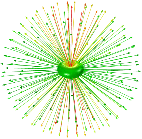
Ray release based on the far-field radiation pattern of a dipole antenna.