COMSOL 6.4 - The Electromagnetic Waves, Boundary Elements Interface

The interface (

) is used to solve for time-harmonic electromagnetic field distributions. This interface is found under the branch (

) when adding a physics interface,. The formulation is based on the boundary element method (BEM) and is available in 2D and 3D. The physics interface solves the vector Helmholtz equation for piecewise-constant material properties and uses the electric field as dependent variable.

The interface is fully multiphysics enabled and can be coupled seamlessly with the physics interfaces that are based on the finite element method (FEM). This approach allows modeling in a FEM-BEM framework, exploiting the strength of both formulations to the fullest. The BEM-based interface is especially well suited for radiation and scattering problems.

The advantage of the boundary element method is that only boundaries need to be meshed and the degrees of freedom (DOFs) solved for are restricted to the boundaries. This introduces some clear ease-of-use for handling complex geometries. However, the BEM technique results in fully populated or dense matrices that need dedicated numerical methods. The BEM method is so to speak more expensive per DOF than the FEM method, but has fewer DOFs. Assembling and solving these can be very demanding. This means that when solving models of small and medium size, The Electromagnetic Waves, Frequency Domain Interface will often be faster, than solving the same problem with the BEM interface. The challenge for the FEM interface is to set up open boundaries, for example, using Perfectly Matched Layers (PMLs) in an efficient way. When the geometries are complex or two structures are far apart, large air domains need to be meshed. This costs a lot on the computational side as the frequency is increased.

For large models (problems that contain many wavelengths, at high frequency or for large domains) the stabilized formulation option (see Stabilization) ensures efficient convergence at the cost of some additional degrees of freedom. For low to medium frequencies (small to medium models), running without stabilization is more efficient. The stabilized formulation only gives a benefit in computing time for the large models.

For this physics interface, the maximum mesh element size should well resolve the complex electric field on the boundaries. Thus, if the wave propagates tangentially to the boundary, the maximum mesh size should be a fraction of the wavelength. However, if the wave propagates essentially in the normal direction to the boundary, the maximum mesh element size can be larger. The physics interface supports the Frequency Domain study types. The Frequency Domain study type is used for source driven simulations for a single frequency or a sequence of frequencies.

	In the COMSOL Multiphysics Reference Manual see the Theory for the Boundary Elements PDE section for more information about the Boundary Element Method.

When this physics interface is added, these default nodes are also added to the — , , and . Then, from the toolbar, add other nodes that implement, for example, boundary conditions. You can also right-click to select physics features from the context menu.

	If both The Electromagnetic Waves, Frequency Domain Interface and The Electromagnetic Waves, Boundary Elements Interface are available, the Electric Field Coupling node is available from the Multiphysics menu in the Physics toolbar or by right-clicking the Multiphysics Couplings node in Model Builder.
	The Electromagnetic Waves, Frequency Domain Interface and The Electromagnetic Waves, Boundary Elements Interface can also be coupled by using the same name for the dependent variable for both interfaces. Then Electric Field Coupling is not needed. How to set the name for the dependent variable is described in the Dependent Variables section.

The physics-controlled mesh only defines mesh settings for the boundaries. It is controlled from the window for the node (if the is ). In the table in the section, find the physics interface in the column and select or clear the checkbox in the column on the same row for enabling (the default) or disabling contributions from the physics interface to the physics-controlled mesh.

When the checkbox for the physics interface is selected, this invokes a parameter for the maximum mesh element size in free space. The physics-controlled mesh automatically scales the maximum mesh element size as the wavelength changes in different dielectric and magnetic regions.

When the checkbox is selected for the physics interface, in the section for the physics interface below the table, choose one of the four options for the — (the default), , , or . When is selected, 1/5 of the vacuum wavelength from the highest frequency defined in the study step is used for the maximum mesh element size. For the option , enter a suitable . For example, 1/5 of the vacuum wavelength or smaller. When is selected, enter the highest frequency intended to be used during the simulation. The maximum mesh element size in free space is 1/5 of the vacuum wavelength for the entered frequency. For the option, enter the smallest vacuum wavelength intended to be used during the simulation. The maximum mesh element size in free space is 1/5 of the entered wavelength.

The maximum mesh element size in dielectric media is equal to the maximum mesh element size in vacuum divided by the square root of the product of the relative permittivity and permeability.

	In the COMSOL Multiphysics Reference Manual see the Physics-Controlled Mesh section for more information about how to define the physics-controlled mesh.

The is the default physics interface name.

The is used primarily as a scope prefix for variables defined by the physics interface. Refer to such physics interface variables in expressions using the pattern <name>.<variable_name>. In order to distinguish between variables belonging to different physics interfaces, the name string must be unique. Only letters, numbers, and underscores (_) are permitted in the field. The first character must be a letter.

The default (for the first physics interface in the model) is embe.

The toolbar buttons enable faster and easier modeling by analyzing the geometry and configuring appropriate physics features and settings.

The button creates a half-geometry and assigns PEC- or PMC-type properties, depending on the user’s selection. There are six available options. These buttons operate only in 3D.

From the list, select any of the options — , , , or (the default). The geometric entity list displays the selected domain entity numbers. Edit the list of selected domain entity numbers using the selection toolbar buttons to the right of the list or by selecting the geometric entities in the window. Entity numbers for voids can be entered by clicking the Paste (

) button in the selection toolbar and supplying the entity numbers in the dialog. The entity number for the infinite void is 0, and finite voids have negative entity numbers.

Selections can also be entered using the window, available from the menu in the toolbar.

	For more information about making selections, see Working with Geometric Entities in the COMSOL Multiphysics Reference Manual.

This section is available for 2D components.

Select the — , , or . Select:

From the list, select whether to solve for the (the default) or the .

For select a according to the following table:

Table 4-3: Background wave type based on component dimension.
Component	Background wave type
2D	User defined (default), Gaussian beam
3D	User defined (default), Gaussian beam, Linearly polarized plane wave

	The scattered field formulation supports both metallic PEC scatterers and dielectric scatterers. Notice that a Wave Equation, Electric can be active on multiple domains provided that each material parameter (Relative permittivity, Relative permeability, and Electric conductivity) has the same constant value in all the selected domains. In brief, there needs to be a Wave Equation, Electric node for each dielectric material. When multiple Wave Equation, Electric nodes exist, the Infinite void selection needs to correspond to the first Wave Equation, Electric node and cannot coexist with other domain selections.

Enter the component expressions for the Eb (SI unit: V/m). The entered expressions must be differentiable.

	Notice that expressions including coupling operators are not differentiable and cannot be used as background fields.

For select the — (the default) or .

When selecting , the Gaussian beam background field is a solution to the paraxial wave equation, which is an approximation to the Helmholtz equation solved for by the interface. The approximation is valid for Gaussian beams that have a beam radius that is much larger than the wavelength. Since the paraxial Gaussian beam background field is an approximation to the Helmholtz equation, for tightly focused beams, you can get a nonzero scattered field solution, even if you do not have any scatterers. The option means that the electric field for the Gaussian beam is approximated by an expansion of the electric field into a number of plane waves. Since each plane wave is a solution to the Helmholtz equation, the plane wave expansion of the electric field is also a solution to the Helmholtz equation. Thus, this option can be used also for tightly focused Gaussian beams.

If the beam spot radius is smaller than the wavelength, evanescent plane waves need to be included in the expansion. The evanescent waves decay exponentially in the propagation direction, why it only makes sense to model such tightly focused beams if the focal plane coincides with the input boundary. If the focal plane is located inside the modeled domain, the field can be dominated by the exponentially decaying evanescent waves. Those waves can have a very high field strength before the focal plane even though they only provide a small contribution to the field at the focal plane.

For select — (the default) or . For also check , to include evanescent waves in the plane wave expansion. For also enter values for the Nk (the default value is 13) and kt,max (SI unit: rad/m, default value is (2*(sqrt(2*log(10))))/embe.w0). Use an odd number for the Nk to make sure that a wave vector pointing in the main propagation direction is included in the plane-wave expansion. The Nk specifies the number of wave vectors that will be included per transverse dimension. So for 3D the total number of wave vectors will be Nk·Nk.

	Evanescent waves are included in the plane wave expansion if the Maximum transverse wave number kt,max is larger that the specified Wave number k. When the Wave vector distribution type is set to Automatic, evanescent waves are included in the expansion if the Allow evanescent waves checkbox is selected.

A plane wave expansion with a finite number of plane waves included will make the field periodic in the plane orthogonal to the main propagation direction. If the separation between the transverse wave vector components, given by 2kt,max/(Nk − 1), is too small, replicas of the Gaussian beam background field can appear. To avoid that, increase the value for the Nk.

The number of plane waves included in the expansion can be quite large, especially for 3D. For instance, using the default settings, 2·13·13 = 338 plane waves will be included (the factor 2 accounts for the two possible polarizations for each wave vector). Thus, initializing the plane-wave expansion for the Gaussian beam background field can take some time in 3D.

For more information about the Gaussian beam theory, see Gaussian Beams as Background Fields and Input Fields.

Define the Gaussian beam background field using the parameters below:

•

Enter the component expressions for the ETbg0 (SI unit: V/m) if the is . Notice that this is the transverse Gaussian beam amplitude in the focal plane. When the is set to the background field is always orthogonal (transverse) to . However, when the is set to , the background field amplitude can also have a component in the propagation direction. Specify here only the field amplitude components that are orthogonal to the propagation direction. COMSOL computes automatically the component in the propagation direction, if needed.

•

If the is set to , enter the (SI unit: W in 2D axisymmetry and 3D and W/m in 2D) and the component expressions for the ETbg0 (SI unit: V/m).

•

Enter a k (SI unit: rad/m). The default is embe.k0 rad/m. The wave number must evaluate to a value that is the same for all the domains the scattered field is applied to. Setting the k to a positive value means that the wave is propagating in the positive x-, y-, or z-axis direction, whereas setting the k to a negative value means that the wave is propagating in the negative x-, y-, or z-axis direction.

The initial background wave is predefined as E0 = exp(−jkxx)z. This field is transformed by three successive rotations along the roll, pitch, and yaw angles, in that order. For a graphic representation of the initial background field and the definition of the three rotations, compare with Figure 4-1 below.

•

Enter a (SI unit: rad), which is a right-handed rotation with respect to the +y direction. The default is 0 rad, corresponding to the initial direction of propagation pointing in the +x direction.

Figure 4-8: Schematic of the directions for the wave vector k, the electric field E0, and the roll, pitch, and yaw rotations. The top image represents an initial wave propagating in the x direction with a polarization along the z direction.

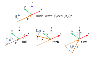
Symmetry planes are normal to the Cartesian coordinate axes. For 0, 0, and 0, select (the default), , or , respectively. For the option or , enter an axis coordinate value of the symmetry plane (SI unit: m).

Select the checkbox to enable the port sweep. When selected, this invokes a parametric sweep over the ports in addition to the frequency sweep already added. The generated lumped parameters are in the form of an S-parameter matrix.

For enter a to assign a specific name to the parameter that controls the port number solved for during the sweep. Before making the port sweep, the parameter must also have been added to the list of parameters in the section of the node under the node. This process can be automated by clicking the button. The button helps add a necessary port sweep parameter and a study step in the last study node. If there is already a study step, the sweep settings are adjusted for the port sweep. Select and the S-parameters are subject to . Click to locate the file, or enter a filename and path. Select an : , , or .

Enter a Zref (SI unit: Ω) that is used only for the header in the exported Touchstone file. The default is 50 Ω.

To display this section, click the button (

) and select in the dialog.

For large models (problems that contain many wavelengths, at high frequency or for large domains) enable the option (enable by default) to ensure efficient convergence at the cost of some additional degrees of freedom.

When is selected, a text field for the is enabled with the default value sqrt(abs(embe.k[m])). This is a parameter that should scale inversely with the wavelength. The default gives good performance in most cases.

To display this section, click the button (

) and select in the dialog.

	For more information about the Far Field Approximation settings, see Far-Field Approximation Settings in the COMSOL Multiphysics Reference Manual.

When is selected, a text field for the is enabled with the default value ((2*pi)/embe.k0)/10 (one tenth of a wavelength). For problems having a wide distribution of mesh element sizes, including mesh elements that are much smaller than the wavelength, a smaller value for this parameter may make the iterative solver convergence faster.

Using a smaller value for this parameter, may make problems having a large distribution of mesh element sizes, including mesh elements that are much smaller than the wavelength, converge faster with the iterative solver. However, a smaller value use more memory.

To display this section, click the button (

) and select in the dialog.

	For more information about the Quadrature settings, see Quadrature in the COMSOL Multiphysics Reference Manual.

From the list, choose from predefined options for the boundary element discretization order for the electric field variable and the flux field (magnetic field) variable, respectively. The predefined options represent the suitable combinations of element orders such as (the default). For more information about the section, see Settings for the Discretization Sections in the COMSOL Multiphysics Reference Manual.

The dependent variables (field variables) are for the E and its components (in the fields). The name can be changed but the names of fields and dependent variables must be unique within a model.