The Electromagnetic Waves, Asymptotic Scattering (ewas) interface (

), found under the
Radio Frequency branch (

) when adding a physics interface, is used for quick studies of the far-field response of a 3D or 2D object to a given background field. The physics interface sets up a surface electric background field for the far-field transformation, using the Stratton–Chu formula, performed in the postprocessing.
When this physics interface is added, these default nodes are also added to the Model Builder:
Asymptotic Scattering,
Far-Field Calculation, and
Initial Values. No additional boundary feature is needed in general. However, from the
Physics toolbar, a new
Far-Field Calculation can be added to process the far-field calculation on user-defined boundary selections. You can also right-click
Electromagnetic Waves, Asymptotic Scattering to select physics features from the context menu.
The Label is the default physics interface name.
The Name is used primarily as a scope prefix for variables defined by the physics interface. Refer to such physics interface variables in expressions using the pattern
<name>.<variable_name>. In order to distinguish between variables belonging to different physics interfaces, the
name string must be unique. Only letters, numbers, and underscores (_) are permitted in the
Name field. The first character must be a letter.
The default Name (for the first physics interface in the model) is
ewas.
The physics-controlled mesh is controlled from the Mesh node’s
Settings window (if the
Sequence type is
Physics-controlled mesh). In the table in the
Physics-Controlled Mesh section, find the physics interface in the
Contributor column and select or clear the checkbox in the
Use column on the same row for enabling (the default) or disabling contributions from the physics interface to the physics-controlled mesh.
When the Use checkbox for the physics interface is selected, this invokes a parameter for the maximum mesh element size in free space. The physics-controlled mesh automatically scales the maximum mesh element size as the wavelength changes.
When the Use checkbox is selected for the physics interface in the section for the physics interface below the table, choose one of the four options for the
Maximum mesh element size control parameter —
From study (the default),
User defined,
Frequency, or
Wavelength. When
From study is selected, 1/5 of the vacuum wavelength from the highest frequency defined in study step is used for the maximum mesh element size. For the option
User defined, enter a suitable
Maximum element size in free space. For example, 1/5 of the vacuum wavelength or smaller. When
Frequency is selected, enter the highest frequency intended to be used during the simulation. The maximum mesh element size in free space is 1/5 of the vacuum wavelength for the entered frequency. For the
Wavelength option, enter the smallest vacuum wavelength intended to be used during the simulation. The maximum mesh element size in free space is 1/5 of the entered wavelength.
For Scattered field select a
Background wave type according to the following table:
Enter the component expressions for the Background electric field Eb (SI unit: V/m). The entered expressions must be differentiable.
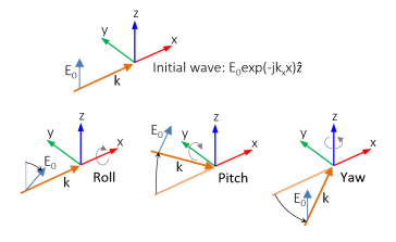
The initial background wave is predefined as E0 = exp(
−jkxx)
z. This field is transformed by three successive rotations along the roll, pitch, and yaw angles, in that order. For a graphic representation of the initial background field and the definition of the three rotations; compare with
Figure 4-1 below.
The dependent variables (field variables) are for the Electric field E and its components (in the
Electric field components fields). The name can be changed but the names of fields and dependent variables must be unique within a model.
Select the shape order for the Electric field dependent variable —
Linear,
Quadratic (the default), or
Cubic. For more information about the
Discretization section, see
Settings for the Discretization Sections in the
COMSOL Multiphysics Reference Manual.