Introduction
The RF Module is used by engineers and scientists to understand, predict, and design electromagnetic wave propagation and resonance effects in high-frequency applications. Simulations of this kind result in more powerful and efficient products and engineering methods. It allows users to quickly and accurately predict electromagnetic field distributions, transmission, reflection, and power dissipation in a proposed design. Compared to traditional prototyping, it offers the benefits of lower cost and the ability to evaluate and predict phenomena that cannot be measured directly in experiments. It also allows the exploration of operating conditions that would destroy a real prototype or be hazardous.
This module covers electromagnetic fields and waves in two- and three-dimensional space along with traditional circuit-based modeling of passive and active devices. All modeling formulations are based on Maxwell’s equations or subsets and special cases of these together with material constitutive relations for propagation in various media. The modeling capabilities are accessed via predefined physics interfaces, referred to as Radio Frequency (RF) interfaces, which allow you to set up and solve electromagnetic models. The RF interfaces cover the modeling of electromagnetic fields and waves in frequency domain, time domain, eigenfrequency, and mode analysis.
Under the hood, the RF interfaces formulate and solve the differential form of Maxwell’s equations together with the initial and boundary conditions. The equations are solved using the finite element method with numerically stable edge element discretization in combination with state-of-the-art algorithms for preconditioning and solution of the resulting sparse equation systems. The results are presented using predefined plots of electric and magnetic fields, S-parameters, power flow, and dissipation. You can also display your results as plots of expressions of the physical quantities that you define freely, or as tabulated derived values obtained from the simulation.
The workflow consists of the following steps: define the geometry, select materials, select a suitable RF interface, define boundary and initial conditions, define the finite element mesh, select a solver, and visualize the results. All these steps are accessed from the COMSOL Desktop. The solver selection step is usually carried out automatically using default settings, which are tuned for each specific RF interface.
The RF Module’s application library describes the physics interfaces and the different features through tutorial and benchmark examples for the different formulations. The library provides a wide range of examples, including antenna arrays, couplers and power dividers, electromagnetic interference and compatibility (EMI/EMC) applications, electrostatic discharge (ESD) and lightning surge studies, ferrimagnetic devices, filters, microwave heating, passive components, scattering and radar cross-section (RCS) analysis, and transmission lines and waveguides. It also provides tutorials for education and verification models for benchmarking the RF interfaces.
This introduction is intended to give you a jump start in your modeling work. It has examples of the typical use of the RF Module, a list of the physics interfaces with a short description, and a tutorial model that introduces the modeling workflow.
The Use of the RF Module
The RF interfaces are used to model electromagnetic fields and waves in high frequency applications. The latter means that it covers the modeling of devices that are above about 0.1 electromagnetic wavelength in size. Thus, it may be used to model microscale devices or human size devices operating at frequencies above 10 MHz.
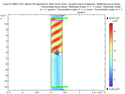
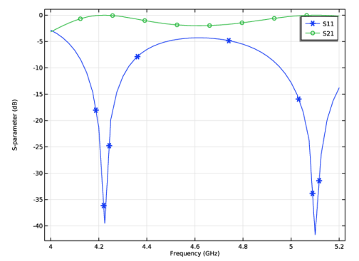
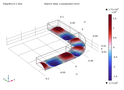
RF simulations are frequently used to extract S-parameters characterizing the transmission and reflection of a device. Figure 1 shows the electric field distribution in a dielectric loaded H-bend waveguide component. A rectangular TE10 waveguide mode is launched into the inport at the near end of the device and is absorbed by the outport at the far end. The bend region is filled with silica glass.
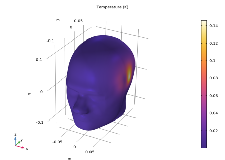
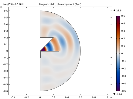
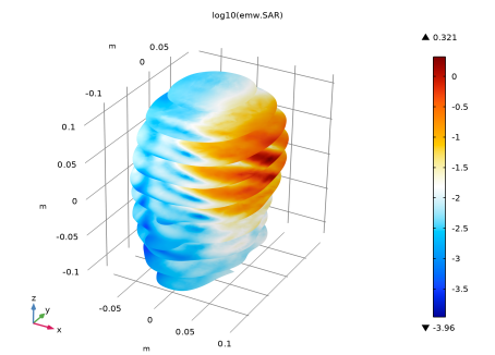
Figure 1: Electric field distribution in a dielectric loaded H-bend waveguide. From the application library, H-Bend Waveguide 3D.
The transmission and reflection of the device are expressed quantitatively by the S-parameters, shown in Figure 2.
Figure 2: The S-parameters, on a dB scale, as a function of the frequency.
The S-parameters are, by themselves, useful performance measures of a device. They can also be exported as a Touchstone file for further use in system simulations.
In Figure 3 and Figure 4, an application library entry for the RF Module shows how a human head absorbs a radiated wave from an antenna held next to an ear. The temperature is increased by the absorbed radiation.
Figure 3: The local increase in temperature in a human head due to absorption of electromagnetic energy from an antenna held next to the ear. From the application library entry Absorbed Radiation (SAR) in the Human Brain.
The SAR (specific absorption rate) value is of specific interest to designers of mobile telephones and is readily obtained from the simulation.
Figure 4: Log-scale slice plot of the local specific absorption rate (SAR) in a human head.
The RF Module also offers a comprehensive set of features for 2D modeling including both source driven wave propagation and mode analysis. Figure 5 shows mode analysis of a step-index profile optical fiber.
Figure 5: The surface plot visualizes the longitudinal component of the electric field in the fiber core. From the application library entry Step Index Fiber.
Both in 2D and 3D, the analysis of periodic structures is popular. Figure 6 is an example of a plane wave incidence on a wire grating with a dielectric substrate.
Figure 6: Electric field norm for TE incidence at π/5. From the application library entry Plasmonic Wire Grating.
It is also possible to perform body-of-revolution (BOR) simulations in 2D axisymmetry. Figure 7 illustrates the modeling of a monoconical antenna with a coaxial feed.
Figure 7: Axisymmetric model of a monoconical antenna with a coaxial feed. The azimuthal component of the magnetic field is shown. From the application library entry Conical Antenna.
The RF Module has a vast range of tools to evaluate and export the results, for example, evaluation of far-field, feed impedance, and scattering matrices (S-parameters). S-parameters can be exported in the Touchstone file format.
Full-wave electromagnetic field modeling can also be combined with circuit-based modeling. This is an ideal basis for design, exploration, and optimization. More complex system models can be created using circuit-based modeling while maintaining links to full field models for key devices in the circuit allows for design innovation and optimization on both levels.