Study 1
The flow field can be assumed to be independent of time, it is calculated in a first stationary step and then used as input for the heat transport in the subsequent time-dependent step.
Step 1: Stationary
1
In the Model Builder window, under Study 1 click Step 1: Stationary
.
2
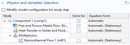
In the Settings window for Stationary, locate the Physics and Variables Selection section.
3
In the table, clear the Solve for checkboxes for Heat Transfer in Solids and Fluids and for Nonisothermal Flow 1.
Time Dependent
1
In the Study toolbar, click Study Steps
and choose Time Dependent
.
2
In the Settings window for Time Dependent, locate the Physics and Variables Selection section. Clear the Solve for checkbox for Free and Porous Media Flow, Brinkman.
3
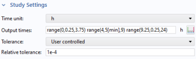
Locate the Study Settings section. From the Time unit list, choose h (hours).
4
In the Output times text field, type
range(0,0.25,3.75) range(4,5[min],9) range(9.25,0.25,24)
.
The time stepping is chosen such that the phase change is resolved properly.
5
From the Tolerance list, choose User controlled.
6
In the Relative tolerance text field, type
1e-4
.
A tighter tolerance improves the accuracy of the solution which is necessary for resolving all physical effects including the phase change properly.
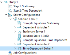
Solution 1
1
In the Study toolbar, click Show Default Solver
.
2
In the Model Builder window, expand the Solution 1 node, then click Time-Dependent Solver 1
.
3
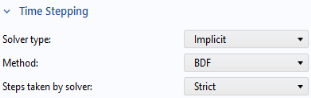
In the Settings window for Time-Dependent Solver, click to expand the Time Stepping section.
4
From the Steps taken by solver list, choose Strict.
This forces the solver to use at least the time steps specified above.