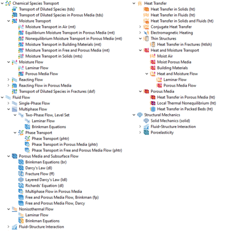
 Chemical Species Transport Chemical Species Transport |
|||||
 |
|||||
 |
|||||
 |
|||||
 Moisture Transport Moisture Transport |
|||||
 |
|||||
 |
|||||
 |
|||||
 |
|||||
 |
|||||
 |
|||||
 Moisture Flow Moisture Flow |
|||||
 |
|||||
 |
|||||
 Reacting Flow Reacting Flow |
|||||
 |
|||||
 Reacting Flow in Porous Media Reacting Flow in Porous Media |
|||||
 |
|||||
 Fluid Flow Fluid Flow |
|||||
 Single-Phase Flow Single-Phase Flow |
|||||
 |
|||||
 |
|||||
 Multiphase Flow Multiphase Flow |
|||||
 Two-Phase Flow, Level Set Two-Phase Flow, Level Set |
|||||
 |
|||||
 Phase Transport Phase Transport |
|||||
 |
|||||
 |
|||||
 |
|||||
 Porous Media and Subsurface Flow Porous Media and Subsurface Flow |
|||||
 |
|||||
 |
|||||
 |
|||||
 |
|||||
 |
|||||
 |
|||||
 |
|||||
 |
|||||
 Nonisothermal Flow Nonisothermal Flow |
|||||
 |
|||||
 Heat Transfer Heat Transfer |
|||||
 |
|||||
 |
|||||
 |
|||||
 Thin Structures Thin Structures |
|||||
 |
|||||
 Heat and Moisture Transport Heat and Moisture Transport |
|||||
 |
|||||
 |
|||||
 |
|||||
 Heat and Moisture Flow Heat and Moisture Flow |
|||||
 |
|||||
 |
|||||
 Porous Media Porous Media |
|||||
 |
|||||
 |
|||||
 |
|||||
 Structural Mechanics Structural Mechanics |
|||||
 Poroelasticity Poroelasticity |
|||||
 |
|||||
 |
|||||
 |
|||||
 Mathematics Mathematics |
|||||
 |
|||||
 |
|||||
|
2 This physics interface is a predefined multiphysics coupling that automatically adds all the physics interfaces and coupling features required.
|
|||||
|
3 Requires the addition of the Structural Mechanics Module.
4 Requires the addition of the Composite Materials Module and the Structural Mechanics Module.
|
|||||
 ), Fluid Flow (
 ), Heat Transfer (
 ), and Structural Mechanics (
 ), as discussed in the next pages.
 ) simulates chemical species transport through convection (when coupled to fluid flow), diffusion, and reactions, for mixtures where one component, a solvent, is present in excess.
 ) is tailored to model solute transport in saturated and partially saturated porous media. This physics interface characterizes the rate and transport of individual or multiple and interacting chemical species for systems containing fluids, solids, and gases. The equations supply predefined options to describe mass transfer by convection, adsorption, dispersion, diffusion, volatilization, and reactions. You define the convective velocity from either of the included physics interfaces, or you set it to a predefined velocity profile.
 ) under the Reacting Flow branch combines the functionality of the Single-Phase Flow and Transport of Diluted Species interfaces. This multiphysics interface is primarily applied to model flow at low to intermediate Reynolds numbers in situations where the mass transport and flow fields are coupled.
 ) under the Reacting Flow in Porous Media branch combines the Brinkman Equations and the Transport of Diluted Species in Porous Media interfaces. This multiphysics interface is primarily applied to model the transport of diluted reacting mixtures in porous media.
  ) is used to model the transport of a solutes along thin porous fractures, taking into account diffusion, dispersion, convection, and chemical reactions. The fractures are defined by boundaries in 2D and 3D, and the solutes are diluted in a solvent. The mass transport equation solved along the fractures is the tangential differential form of the convection–diffusion–reaction equation. Different effective diffusivity models are available.
 ) is used to compute the relative humidity distribution in air. It simulates moisture transport by vapor convection and diffusion in moist air and the evaporation or condensation on walls.
 ) is used to compute the relative humidity field in porous media. It simulates moisture transport by vapor convection and diffusion in the gas phase, liquid water transport by convection and capillarity in the pores of the media. A Hygroscopic Porous Medium feature with an equilibrium formulation is active by default on all domains.
 ) is used to compute the relative humidity and liquid water saturation fields in porous media. It simulates moisture transport by vapor convection and diffusion in the gas phase, liquid water transport by convection and capillarity in the pores of the media. A Hygroscopic Porous Medium feature with a nonequilibrium formulation is active by default on all domains.
 ) is used to compute the relative humidity field in building materials. It simulates moisture transport by taking into account moisture storage, liquid transport by capillary suction forces.
 ) is used to compute the relative humidity field in all domains, and additionally the liquid water saturation in porous media. It simulates moisture transport by vapor convection and diffusion in the gas phase, liquid water transport by convection and capillarity in the pores of the media. A Moist Air feature is active by default on all domains, and a Hygroscopic porous Medium is added by default with no selection. This interface handles all types of interface between free and porous media, and between two porous media.
 ) is used to compute the relative humidity and moist air pressure in porous media. It simulates moisture transport by vapor convection and diffusion in the gas phase and liquid water transport by convection and capillarity in the pores of the medium.
 ) under the Moisture Flow branch combines all features from the Moisture Transport in Air and Single-Phase Flow interfaces. The Moisture Flow multiphysics coupling is automatically added. The fluid properties may depend on vapor concentration. The physics interface supports low Mach numbers (typically less than 0.3). Similarly to Conjugate Heat Transfer coupling, the moisture transport interface can be coupled with additional turbulence models for the free flow with the use of the CFD Module.
 ) under the Moisture Flow branch combines all features from the Equilibrium Moisture Transport in Porous Media and Brinkman Equations interfaces. The Moisture Flow multiphysics coupling is automatically added. The transport properties can depend on vapor concentration in air. Models can also include moisture transport in building materials.
 ) approximates the Navier–Stokes equations for the case when the Reynolds number is significantly less than 1. This is often referred to as Stokes flow and it is appropriate for use when viscous flow is dominant.
 ) describes fluid motion when turbulences are not present, and the Reynolds number is less than approximately 1000. The physics interface solves the Navier–Stokes equations for incompressible, weakly compressible, or compressible flows where the Mach number (Ma) is less than 0.3.
 ) under the Multiphase Flow branch are used to model two fluids separated by a fluid-fluid interface in a free or a porous medium. The moving interface is tracked in detail using the level set method. The level set method solves additional equations to track the interface location.
 )under the Multiphase Flow branch is used to simulate the transport of multiple immiscible phases in free flow. This interface solves for the averaged volume fractions of the phases.
 ) interface is used to simulate the transport of multiple immiscible phases through a porous medium. This interface solves for the averaged volume fractions (also called saturations in a porous medium) of the phases.
 ) can be used to model transport of an arbitrary number of phases in coupled free and porous media flow. An absolute pressure must be supplied in the porous region and a velocity must be supplied in the free-flow region. Both can be obtained from one of the momentum conservation interfaces or be specified manually.
 ) describes fluid movement through interstices in a porous medium. This physics interface can be used to model low velocity flows, for which the pressure gradient is the major driving force, and the flow is mostly influenced by the frictional resistance within the pores. Its use is within very low flows, or media where the permeability and porosity are very small. You can also set up multiple Darcy’s Law interfaces to model multiphase flows involving more than one mobile phase. The Darcy’s Law interface can also add non-Darcian effects such as Ergun or Forchheimer drag terms, which are important for Reynolds numbers bigger than 100.
 ) is a variant of Darcy’s law that defines the flow along interior boundaries representing fractures within a porous (or solid) medium.
 ) analyzes flow in variably saturated porous media. With variably saturated flow, the permeability changes as fluids move through the medium, filling some pores and draining others. Richards’ equation appears similar to the saturated flow equation set out in Darcy’s Law, but it is notoriously nonlinear due to changes in material properties from unsaturated to saturated conditions. The analytic formulas of van Genuchten and Brooks and Corey are frequently employed with variably saturated flow modeling.
  ) is used to model incompressible, weakly compressible, or compressible flows where the Mach number (Ma) is less than 0.3. You can select the Stokes-Brinkman flow feature to reduce the equations’ dependence on inertial effects, when the Reynolds number is significantly less than one. The Brinkman Equations interface extends Darcy’s law to describe the dissipation of the kinetic energy by viscous shear, similar to the Navier–Stokes equation. The Brinkman Equations interface can also add an Ergun or Forchheimer drag term, which are viscous drags proportional to the square of the velocity. These non-Darcian effects are important for Reynolds numbers bigger than 100.
 ) combines the functionality of the Darcy’s Law and Phase Transport in Porous Media interfaces. This multiphysics interface is intended to model flow and transport of multiple immiscible phases in a porous medium.
 ) is useful for modeling problems where free flow is connected to porous media, such as in fixed-bed reactors and catalytic converters. The Free and Porous Media Flow, Brinkman interface is used over at least two different domains, a free channel and a porous medium. The physics interface adds functionality that allows the equations to be optimized according to the flow properties of the relevant domain. For example, you can select the Stokes-Brinkman flow feature to reduce the equations’ dependence on inertial effects in the porous domain, or just the Stokes’ flow feature to reduce the equations’ dependence on inertial effects in the free channel.
 ) models porous media flow connected to free flow domains. This multiphysics interface couples the Laminar Flow interface with the Darcy’s Law interface over their common boundary.
 ) describes, by default, heat transfer by conduction. The physics interface is also able to account for the heat flux due to translation in solids as well as for solid deformation, including volume or surface changes.
 ) accounts for conduction and convection in gases and liquids as the default heat transfer mechanisms. The coupling to the flow field in the convection term is automatically set when the Nonisothermal Flow multiphysics coupling is used. Otherwise, it may be entered manually in the physics interface, or it may be selected from a list that couples heat transfer to an existing fluid flow interface.
 ) contains solids and fluids domains by default. It is aimed to simplify the setup of models where capabilities of Heat Transfer in Solids interface (
 ) and Heat Transfer in Fluids interface (
 ) are used, in particular in conjugate heat transfer applications.
 ) combine features from the Heat Transfer and Single-Phase Flow interfaces to describe heat transfer in solids and fluids and nonisothermal flow in fluids. The heat transfer process is tightly coupled with the fluid flow problem via a predefined multiphysics coupling. Additional turbulence models for the free flow are available with the use of the CFD Module.
 ) under the Thin Structures branch (
 ) describes heat transfer in fractures and thin porous media. It provides efficient models defined at the boundaries level representing thin three-dimensional domains. The simplest model assumes that the temperature changes through the fracture thickness can be neglected, while the general model computes the temperature variation across the fracture.
 ) under the Heat and Moisture Transport branch combines the Heat Transfer in Moist Air interface (
 ) with the Moisture Transport in Air interface (
 ). It is used to simulate the coupling between heat transfer and vapor transport in air and the evaporation and condensation on walls.
 ) combines the Heat Transfer in Moist Porous Media and Equilibrium Moisture Transport in Porous Media interfaces. It is used to simulate the coupling between heat transfer and moisture transport in liquid and gas phases in the pores of the medium.
 ) combines the Heat Transfer in Building interface (
 ) with the Moisture Transport in Building Materials interface (
 ). It can be used to model different moisture variations phenomena in building components such as drying of initial construction moisture, condensation due to migration of moisture from outside to inside, or moisture accumulation by interstitial condensation due to diffusion.
 ) combines the heat conduction and convection in a solid-fluid system. This physics interface provides mixing rules for calculating the effective heat transfer properties, expressions for heat dispersion in porous media. Dispersion is caused by the tortuous path of the liquid in the porous medium, which would not be described if only the mean convective term was taken into account. This physics interface may be used for a wide range of porous materials, from porous structures to the simulation of heat transfer in soils and rocks, and also to model heat transfer in fractures.
 ) implements a macroscale model designed to simulate heat transfer in porous media where the temperatures in the porous matrix and the fluid are not in equilibrium. It differs from simpler macroscale models for heat transfer in porous media where the temperature difference of the solid and fluid are neglected. The absence of thermal equilibrium can result from fast transient changes, but it can also be observed in stationary cases. Typical applications are rapid heating or cooling of a porous medium using a hot fluid or internal heat generation in one of the phases (due to inductive or microwave heating, exothermic reactions, and so on). This is observed in nuclear devices, electronics systems, or fuel cells for example.
 ) provides a multiscale model for heat transfer in a porous medium where the local thermal equilibrium is not assumed between the pellets of a packed bed and the fluid phase, and where the temperature variation inside the pellets is taken into account. A temperature field is defined for each phase, pellets and fluid of the porous medium, and the heat transfer between them is accounted for. The microscale pellets temperature field depends on the radial coordinate of each pellet.
 ) combines a transient formulation of Darcy’s law with a linear elastic material included in the Solid Mechanics interface. The poroelasticity coupling means that the pore fluid affects the compressibility of the porous medium, as well as changes in volumetric strains affect the porosity and the fluid flow.