The Fluid Flow >
Single-Phase Flow branch (

) when adding a physics interface includes the Creeping Flow, Viscoelastic Flow and Rotating Machinery, Laminar Flow interfaces.
The Creeping Flow Interface (

) approximates Navier–Stokes equations for very low Reynolds numbers. This is often referred to as Stokes flow and is applicable when viscous effects are dominant, such as in very small channels or microfluidics devices. The Creeping Flow interface also allows for simulation of inelastic non-Newtonian fluids.
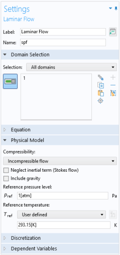
The Laminar Flow Interface (

) is primarily applied to flows at low to intermediate Reynolds numbers. This physics interface solves Navier–Stokes equations for incompressible, weakly compressible, and compressible flows (up to Mach 0.3). The Laminar Flow interface also allows for simulation of inelastic non-Newtonian fluids.
The Rotating Machinery, Laminar Flow Interface (

) combines the Laminar Flow interface and a Rotating Domain and is applicable to fluid-flow problems where one or more of the boundaries rotate (for example, in mixers and around propellers). The physics interface supports incompressible, weakly compressible, and compressible (Mach < 0.3) laminar flows of Newtonian and inelastic non-Newtonian fluids.
The Viscoelastic Flow Interface (

) is used to simulate incompressible isothermal flow of viscoelastic fluids. It solves the continuity equation, the momentum equation, and a constitutive equation that defines the elastic stresses. There are several predefined models for the elastic stresses: Oldroyd-B, FENE-P, Giesekus, LPTT, and EPTT.