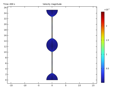
Results
After the computation, the velocity plot for the final time will be shown
Continue with a visualization of the filament shape at selected times (
Figure 10
).
Shape
1
In the Model Builder window, right-click Velocity (vef) and choose Duplicate.
2
In the Settings window for 2D Plot Group, type Shape in the Label text field.
Surface
1
In the Model Builder window, expand the Shape node, then click Surface.
2
In the Settings window for Surface, locate the Expression section.
3
In the Expression text field, type 1.
4
Locate the Coloring and Style section. From the Coloring list, choose Uniform.
5
From the Color list, choose Black. The plot shows the shape at the last time step, t=300.
6
Right-click Surface and choose Solution Array.
7
In the Settings window for Solution Array, locate the Data section.
8
From the Time selection list, choose From list.
9
In the Times (s) list, choose 0, 20, 30, 100, and 300 to plot the shape evolution at different times.
10
In the Shape toolbar, click Plot.
Now, plot the minimum filament radius.
Line Minimum 1
1
In the Results toolbar, click Numerical
and then More Derived Values
and choose Minimum > Line Minimum.
2
Select the Boundary 4 only.
3
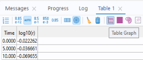
In the Settings window for Line Minimum, locate the Expressions section, enter
log10(r)
.
4
Locate the Data section. From the Dataset list, choose Study 1/Remeshed Solution 1 (sol2).
5
Click
Evaluate.
Table
The result appears in the Table window at the bottom of the COMSOL Desktop. Click Table Graph in the window toolbar.