COMSOL 6.4 - Global Definitions

Global Definitions

Next, define the geometry and process condition parameters. To streamline this step, you can load the model parameters directly from a text file.

1

In the Home toolbar click Parameters

and select Parameter 1

On Linux and Mac, the Home toolbar refers to the specific set of controls near the top of the Desktop.

2

Load from File.

3

Browse to the model’s Application Libraries folder and double-click the file slot_die_coating_2d_parameters.txt.

Follow the steps below to calculate the power-law fluid model parameters using measured apparent-viscosity vs. shear-rate data.

Least-Squares Fit 1 (lsq1_fun1)

1

In the toolbar, click

and choose .

2

In the window for , locate the section.

3

.

4

Browse to the model’s Application Libraries folder and double-click the file slot_die_coating_2d_viscosity_input.txt.

5

Locate the section. In the table, click to select the cell at row number 1 and column number 1.

6

In the text field, type gammadot.

7

In the text field, type 1.

8

In the table, click to select the cell at row number 2 and column number 1.

9

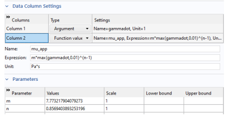
In the text field, type mu_app.

10

In the text field, type m*max(gammadot,0.01)^(n-1).

11

In the text field, type Pa*s.

12

Locate the section. In the table, enter the following settings:


Parameter	Values	Scale	Lower bound	Upper bound
m	1	1
n	1	1

13

. The computed parameter values from the least-squares fit appear in the Parameters table.

14

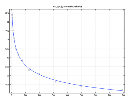
to see how close data points are to the fitted function.

Create a step function to use for ramping up the inlet velocity. To improve convergence, define a smoothing transition zone to gently increase the inlet velocity from zero.

1

In the Home toolbar, click

Functions and choose Global > Step

2

Locate the Parameters section. In the Location text field, type 0.01.

3

Click to expand the Smoothing section. In the Size of transition zone text field, type 0.02.