|
|
|||||
|
|
|||||
|
|
|||||
|
|
|||||
|
|
|||||
|
|
|||||
|
|
|||||
|
|
|||||
|
|
|||||
|
|
|||||
|
|
|||||
|
|
|||||
|
|
|||||
|
|
|||||
|
|
|||||
|
|
|||||
|
|
|||||
|
|
|||||
|
|
|||||
|
|
|||||
|
|
|||||
|
|
|||||
|
|
|||||
|
|
|||||
|
|
|||||
|
|
|||||
|
|
|||||
|
|
|||||
|
|
|||||
|
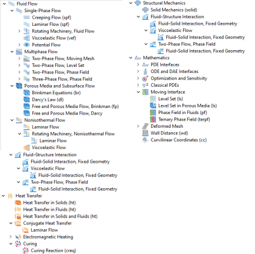
Laminar Flow(2)
|
|
||||
|
|
|||||
|
|
|||||
|
|
|||||
|
|
|||||
|
|
|||||
|
|
|||||
|
|
|||||
|
|
|||||
|
|
|||||
|
|
|||||
|
|
|||||
|
|
|||||
|
|
|||||
|
|
|||||
|
|
|||||
|
|
|||||
|
|
|||||
|
2 This physics interface is a predefined multiphysics coupling that automatically adds all the physics interfaces and coupling features required.
|
|||||