Results
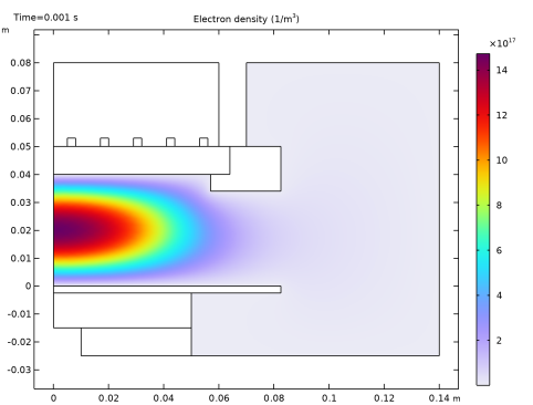
There are three default plots generated, one for the electron number density, one for the electron temperature and one for the electrostatic potential. After the model has solved, the default plot is of the electron density. The peak electron density occurs at the center of the reactor, underneath the RF coil. The electron density in this case is high enough to cause some shielding of the azimuthal electric field.
1
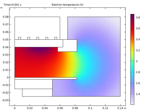
To view the electron temperature, click on the Electron Temperature (plas) plot group
.
The electron “temperature” is highest directly underneath the coil, which is where the bulk of the power deposition occurs.
2
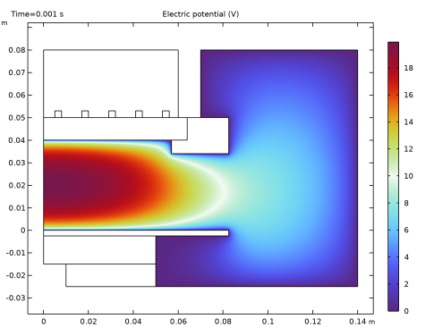
To view the electric potential, click on the Electric Potential (plas) plot group
.
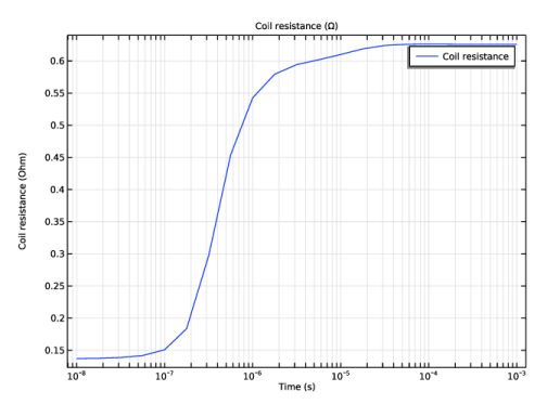
Now add a global plot for the coil resistance. This is defined as the real part of the total voltage drop over the coil divided by the current.
3
In the Model Builder window, right-click Results and choose 1D Plot Group
.
4
Right-click Results > 1D Plot Group 6 and choose Global
.
5
In the Global settings window, locate the y-Axis Data section. Click Replace Expression
. Select Magnetic Fields > Coil Parameters > Coil Resistance (mf.RCoil_1) from the list.
6
Click the x-Axis Log Scale button
in the Graphics toolbar.
7
Click the Plot button
.
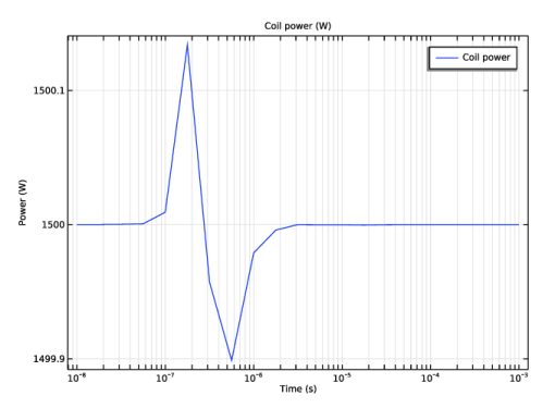
Now add a plot for the total power dissipated in the system. This is one half of the real part of the total voltage drop over the coil multiplied by the applied current.
8
In the Model Builder window, right-click Results and choose 1D Plot Group
.
9
Right-click Results > 1D Plot Group 5 and choose Global.
10
In the Global settings window, locate the y-Axis Data section. Click Replace Expression
. Select Magnetic Fields > Coil Parameters > Coil Power (mf.PCoil_1) from the list.
11
Click the x-Axis Log Scale button
in the Graphics toolbar.
12
Click the Plot button
.
Now you add some additional two dimensional plots.
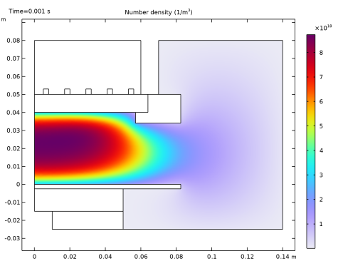
1
In the Model Builder window, right-click Results and choose 2D Plot Group
.
2
Right-click 2D Plot Group 6 and choose Surface
.
3
In the Surface settings window, click Replace Expression
in the upper-right corner of the Expression section. From the menu, choose Plasma (Heavy Species Transport) > Number densities > Number density (plas.n_wAr_1p).
4
Click the Plot button
.
5
Click the Zoom Extents
button in the Graphics toolbar.
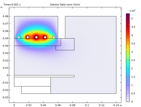
A quick way of creating additional plots is to use the Duplicate option. Now create a plot of the norm of the high frequency electric field.
6
In the Model Builder window, right-click 2D Plot Group 6 and choose Duplicate
.
7
In the Model Builder window, expand the 2D Plot Group 7 node, then click Surface 1
.
8
In the Surface settings window, click Replace Expression
in the upper-right corner of the Expression section. From the menu, choose Magnetic Fields > Electric > Electric field norm (mf.normE).
9
Click the Plot button
.
10
Click the Zoom Extents button
in the Graphics toolbar.
Observe that the electric field is slightly shielded by the plasma. This is due to the skin effect in the plasma. As the electron number density increases, the plasma tends to shield itself from the electric field. Now create a plot of the number density of electronically excited argon atoms.
11
In the Model Builder window, right-click 2D Plot Group 7 and choose Duplicate
.
12
In the Model Builder window, expand the 2D Plot Group 8 node, then click Surface 1
.
13
In the Surface settings window, click Replace Expression
in the upper-right corner of the Expression section. From the menu, choose Plasma (Heavy Species Transport) > Number densities > Number density (plas.n_wArs).
14
Click the Plot button
.
15
Click the Zoom Extents button
in the Graphics toolbar.
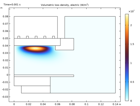
Finally, create a new dataset only active on the plasma domain in order to make it easier to visualize the power deposition into the plasma.
1
In the Model Builder window, expand the Results > Datasets node.
2
Right-click Solution 1 and choose Duplicate
.
3
Right-click Results > Datasets > Study 1/Solution 1 (2) and choose Selection.
4
In the Selection settings window, locate the Geometric Entity Selection section.
5
From the Geometric entity level list, choose Domain.
6
Select Domain 3 only.
7
Deactivate Propagate to lower dimensions.
8
In the Model Builder window, right-click Results and choose 2D Plot Group
.
9
Right-click 2D Plot Group 9 and choose Surface
.
10
In the Surface settings window, locate the Data section.
11
From the Dataset list, choose Study 1/Solution 1(2).
12
Click Replace Expression
in the upper-right corner of the Expression section. From the menu, choose Magnetic Fields > Heating and losses > Volumetric loss density (mf.Qrh).
13
Click the Plot button
.
14
Click the Zoom Extents button
in the Graphics toolbar.
The effect of the shielding of the electric field due to the skin depth of the plasma is also apparent when plotting the power deposition.