For more information about each type, see the interface descriptions in The Pipe Flow Interface section.

Loss coefficients, Ki, for turbulent flow are available in the literature (Ref. 15) and the set predefined in the Pipe Flow interface is reproduced in the table below:

Above, β is the ratio of small to large cross-sectional area. The point friction losses listed above apply for Newtonian fluids. Point losses applying to non-Newtonian flow can be added as user-defined expressions, for instance from (Ref. 16).

For the point pressure loss features Bends, Valves, T-junctions, Y-junctions, n-way junctions, Contractions, and Expansions, the pressure loss can also be specified as a pressure drop Δp directly.

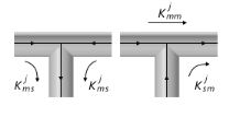
Several options to specify pressure drop across the T-junction branches are available. If the Loss coefficients option is selected, the energy loss between main branches and junction and the energy loss between the side branch and junction are calculated as

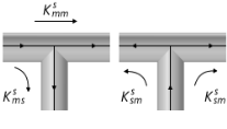
The Loss coefficient with respect to common branch option, which is available for the Pipe Flow interface, implements the loss coefficients according to Ref. 28. The pressure loss for a T-junction is often expressed in terms of the flow in the common branch. For joining flows, the common branch is the collector branch (Figure 2-2, left)

where Kjb,common is the loss coefficient between the branch b and the common branch for joining flows.

For converging (joining) flow, where the collector branch is the side branch (Figure 2-2, left)

For converging flow, where the collector branch is the main branch (Figure 2-2, right)

For diverging (separating) flow, where the supplier branch is the side branch (Figure 2-3, left)

For diverging flow, where the supplier branch is the main branch (Figure 2-3, right)

The mass flow rate ratio qbc = qb/qcommon and the hydraulic diameters ratio are computed automatically. Only junction with sharp corners are considered.

The Loss coefficients, extended model option, that is available for the Pipe Flow interface, allows you to specify the loss coefficient in more details and account for the flow directions. Enter values or expressions for the six dimensionless loss coefficients. See Figure 2-2-Figure 2-3.

Use the Pressure drops option to specify a value or expression for the pressure drop explicitly for each branch respectively:

Predefined loss coefficients are available for both sharp-edged and rounded-edge orifices. (Figure 2-9-Figure 2-10).

The following expression is used for sharp orifices (Ref. 28)

For gently rounded orifice with , the loss coefficient can be found from (Ref. 28)

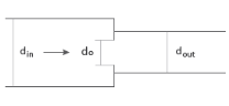
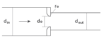
The pressure drop across a control valve can be characterized using flow coefficients such as Cv, Kv, or the resistance coefficient, K. The Cv and Kv coefficients relate the flow rate to the pressure drop under standardized conditions in imperial and metric units, respectively, while the dimensionless coefficient K expresses pressure loss as a function of velocity head. These formulations offer equivalent approaches for assessing valve characteristics. Valve opening refers to the adjustment of the closure element (for example, plug, disc, or ball) relative to the flow passage, which changes the effective flow area. As the valve opens, resistance to flow decreases and capacity increases. Control valve inherent characteristics define the relationship between valve opening and flow capacity under constant pressure drop conditions.

Here, Qv is the volumetric flow rate in (gallons per minute in the U.S. customary system); Cv is the flow coefficient, the flow in gallons per minute that flows through a valve that has a pressure drop of 1 psi across the valve; Δp is the pressure drop across the valve in psi; ρsc is the density of water at 60°F; xfr is the fraction of valve opening; and fsc is the inherit flow characteristic.

To calculate the pressure drop across the valve, the dimensionless loss coefficient K is used:

The relation between the flow coefficient Cv and the dimensionless loss coefficient is given by

where is the numerical value (dimensionless) of the flow coefficient Cv and Ar = 1 in2.

Another commonly used coefficient is the flow factor Kv, which represents the volume of water (in m3/h) flowing through a valve at 16°C with a pressure drop of 1 bar:

Here, R is the rangeability factor, a valve design parameter that is usually in the range [20, 50].

In this case the corresponding pressure drop is calculated to satisfy the flow condition. Using the specified flow rate and the resulting pressure loss, the values of K, Cv, and Kv are computed and available as postprocessing variables. The pressure loss must always be positive, as a valve cannot operate as a pump. However, under certain conditions, the control valve feature may introduce a pressure gain. If this occurs, the values of K, Cv, and Kv are set to −1.

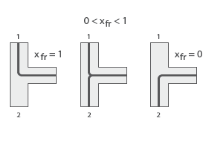
A three-way control valve regulates fluid mixing or diversion between two streams. Its inherent characteristics, determined by port geometry and trim design, define how flow capacity varies with valve position under constant pressure drop conditions (Figure 2-11). The flow is always present in the main branch. When the opening fraction xfr = 1, the flow is fully directed from the main branch to side branch 1. For 0 < xfr < 1, the flow is split between side branch 1 and side branch 2. When xfr = 0, the flow is fully directed from the main branch to side branch 2.

In a 3-way valve, each port can be assigned a different flow characteristic. Pressure loss for each side is calculated in the same way as for a control valve; see Control Valve for details.