High density polyethylene pipe (20 mm diameter) is rolled into sixteen coils. Groups of eight coils are mounted on two sleds. Each coil has a radius of 1 m and a length of approximately 75 m. The coil groups are connected to feed and return piping with a diameter of 50 mm (see Figure 10). The coil groups are 2.4 m in height and sit at the bottom of a pond that is 6 m deep. The total length of the piping is 1446 m.

Above, A (SI unit: m2) is the cross section area of the pipe, ρ (SI unit: kg/m3) is the density, u (SI unit: m/s) is the fluid velocity in the tangential direction of the pipe curve segment, and p (SI unit: N/m2) is the pressure. F (SI unit: N/m3) is a volume force, like gravity.

Gravity can be included explicitly in the model, but since the variation in density is negligible, and the model is not pressure driven, the only effect of including gravity is a change in the total pressure level. It is therefore common modeling practice to exclude gravity from F and interpret the pressure variable as the reduced pressure , where z0 is the datum level of the free liquid surface. This reduces the model complexity and yields the same results. For models where you want to include gravity effects you can add a Volume Force node.

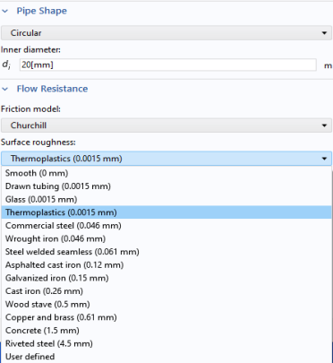
The last two terms of Equation 1 describes the pressure drop due to internal viscous shear and gravity. One of the terms contain the Darcy friction factor, fD, which is a function of the Reynolds number and the surface roughness divided by the hydraulic pipe diameter, e/dh. The Nonisothermal Pipe Flow interface provides a library of built-in expressions for the Darcy friction factor, fD.

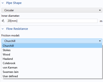
This example uses the Churchill relation (Ref. 1) that is valid for laminar flow, turbulent flow, and the transitional region in between. The Churchill relation is:

The physical properties of water as a function of temperature are directly available from the software’s built-in material library. Inspection of Equation 3 reveals that for low Reynolds numbers (at laminar flow), the friction factor is 64/Re, and for very high Reynolds numbers, the friction factor is independent of Re.

where Cp (SI unit: J/(kg·K)) is the heat capacity at constant pressure, T is the temperature (SI unit: K), and k (SI unit: W/(m·K)) is the thermal conductivity. The second term on the right-hand side of Equation 7 corresponds to friction heat dissipated due to viscous shear. Qwall (SI unit: W/m) is a source/sink term due to heat exchange with the surroundings through the pipe wall:

where Z (m) is the wetted perimeter of the pipe, h (W/(m2·K)) is an overall heat transfer coefficient and Text (K) is the external temperature outside of the pipe.