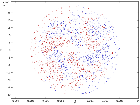
Results
By default you end up in the settings window for the Particle Trajectories (fpt) plot group when the study is complete. Since the default wall condition at the outlet is the Freeze condition, particles are still displayed at the outlet. The color expression of these stopped particles indicates their speed at the time they reached the outlet.
The default Particle Trajectories plot. Particles are colored according to their speed at the final time.
Particle Trajectories (fpt)
1
2
3
Particle Trajectories 1
4
5
6
7
8
9
The at operator evaluates the second input argument at the solution time given by the first. The above expression will return 1 for particles that have a negative initial x-coordinate, or return 0 otherwise.
10
Surface 1
11
12
13
14
15
16
17
18
Surface 2
19
20
21
22
23
24
25
26
27
28
29
30
31
You can also view the trajectories at different times by selecting other solution times in the Settings window for the Particle Trajectories (fpt)  node. You can also cycle through
In the next section, create a copy of this trajectory plot in which the trajectories are rendered as lines instead of points.
Particle Trajectories (fpt) 1
1
2
Particle Trajectories 1
3
4
5
6
7
8
9
10
11
12
Now evaluate the transmission probability using the Particle Counter that was created earlier. For this purpose, transmission probability is defined as the fraction of the released particles to reach the outlet by the final time.
1
2
-
-
3
4
Poincaré Map
One useful way to visualize how particles mix is to use a Poincaré Map plot. The Poincaré map places a colored dot for each particle at the location at which the particle passes through a cut plane (known as a Poincaré section).
The first step is to define the cut planes where the intersections with the particle trajectories will be taken. These cut planes are defined as datasets.
1
2
3
-
-
-
-
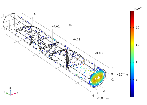
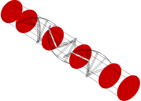
In the Distances text field, type 0.006 0.016 0.026 0.036 0.042.
4
The cut planes will be shown in the Graphics window as shown below.
Cross-sections at which Poincaré maps will be plotted are shown in red.
Poincaré Map
1
2
The plots only display particle positions in each cut plane, but the plot group should still use Particle 1 or one of the Solution datasets as its data source, since this is used to render the dataset edges in the Graphics window.
3
4
5
-
-
In the associated text field, type 0.4. This scaling factor is multiplied by the Point radius expression to determine the size of each point in the plot.
6
7
8
The at operator evaluates an expression at the time specified in the first argument. Here, it is a logical expression based on the initial particle position.
9
-
-
Next add a Surface plot to render the cut planes where the intersection points are computed.
Surface Plot
1
2
3
4
-
-
5
6
In the above figure, the location of the particles at 6 Poincaré sections are shown. The color represents the location of the particle at its initial position. So, particles marked as red had an initial position of x < 0 and particles marked as blue had an initial position of x > 0. The at() operator is used to mark the particles with the color of their initial position. The first Poincaré section (the one furthest to the left in the above figure) clearly indicates which particles start with coordinates of x < 0. As the particles follow the flow field, they begin to mix together. By the end of the mixer, the particles have not mixed completely — there are still significant pockets of only red and only blue particles.
Phase Portrait
Another way to visualize particle positions is using the Phase Portrait plot. A Phase Portrait is a 2D plot in which the axes can be arbitrary expressions in terms of the particle position, velocity, or any other variable that can be evaluated on the particles.
1
2
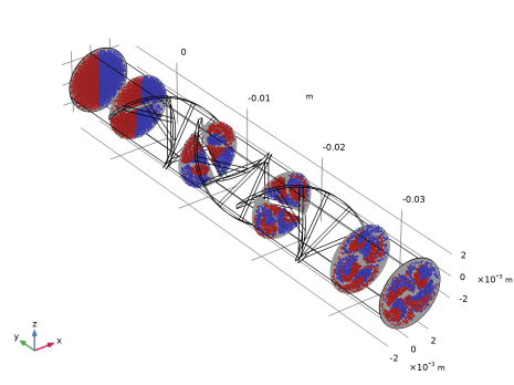
In the Settings window for 2D Plot Group, type Phase Portrait in the Label text field.
3
4
Phase Portrait 1
5
6
7
8
9
10
11
-
-
12
Note: By default the Phase portrait plot scales the coordinate axes so that the plot fits in the Graphics window. This is to ensure that the phase portrait is shown clearly even if the two axes correspond to quantities with vastly different orders of magnitude, like position and momentum. In the present case, both axes represent position components, so by switching to a different view, a 1:1 aspect ratio can be enforced.
13
14
15