Results Processing Tools
Particle Trajectories Plots
A Particle Trajectories plot is available in both 2D
and 3D
. It is created automatically when a Study solving for a particle tracing interface is computed. There are options to set the particle trajectories to be rendered as lines, tubes, or ribbons. It is also possible to render the particles as points, comet tails, arrows, or with a number of ellipses along each trajectory. For models where the number of output times is small, an interpolation option is available that will create smoother looking particle trajectory plots.
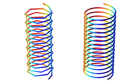
The trajectory of an ion in a uniform magnetic field is plotted with no interpolation (left) and with interpolation (right).
Filters
Visualizing the trajectory of systems with a very large number of particles can consume a lot of computer resources and create cluttered-looking plots in which particles obscure each other from view. It is possible to filter the type of particle and the number of particles which should be rendered. To do this, right click the Particle Trajectories plot type and choose Filter.
The particles can be filtered so that only primary particles secondary particles, or those satisfying a specified logical expression are plotted. It is also possible to plot only a specified fraction or number of particles.
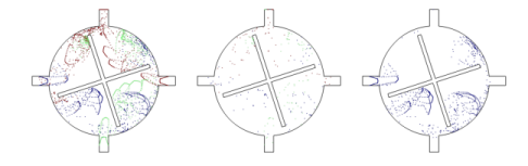
Particle trajectories in a micromixer (left). It is possible to render only a fraction of the particles (middle) and to plot only the particles that are released by a certain inlet using a logical expression (right).
Particle Plots
A Particle plot
can be used to observe the value of a particle property over time. Built-in data series operations can be used, for example, to compute the sum or maximum of an expression over all particles.
Alternatively, the Particle plot can be used to compare two particle properties against each other for all particles at a set of selected time steps.
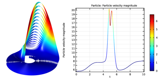
Rossler attractor: 3D plot of particle trajectories (left) and 1D plot of the average speed over time (right).
Poincaré Maps and Phase Portraits
Poincaré maps are available in both 2D
and 3D
. This plot type is useful to visualize the particle trajectories in a plot that represents the position of the particles in a section that is usually transversal to the particle trajectories. The Poincaré map represents the particle trajectories in a space dimension that is one dimension lower than the original particle space.
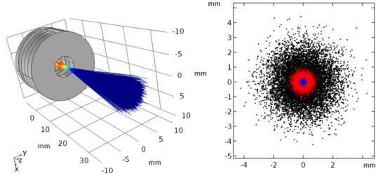
Electrons in a magnetic lens (left). The Poincaré maps (right) show the electron distribution in beam cross-sections at three different axial positions.
Phase portraits
are available as a 2D plot type under More Surface Plots. Use a Phase Portrait plot to visualize large datasets of particle trajectories. The traditional use of a phase portrait is to plot the particle position on the
x
-axis and the particle velocity on the
y
-axis. Each dot in the
xy
-plane represents a particle.
Particle Evaluation
Information about expressions and variables along particle trajectories can be written to the Results Table using the Particle Evaluation
option under Derived Values. Once the data has been written to the results table it can be manipulated and plotted accordingly. There are options to only write data to the table for a fraction or a specific number of particles.
Operations on Particle Data
It is possible to set the source dataset for the Integration
, Average
, Maximum
, and Minimum
to be a Particle
dataset. This allows operations to be performed on the particle dataset, to compute average particle velocity, maximum energy, and so on.
Histograms
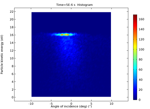
Statistical information about the behavior of the particles is often best visualized with a histogram. The histogram sorts the value of a variable into a specified number of bins. The most obvious application of the histogram is that it allows for visualization of the velocity and energy distribution function of a set of particles.
Information about the ion energy distribution function in a plasma can be visualized using a 2D Histogram.