COMSOL 6.4 - Theory for Time-Dependent Sensitivity

When you enable sensitivity analysis, the time-dependent solvers can compute — in addition to the basic forward solution — the sensitivity of a functional

(2-13)

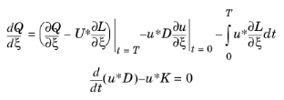
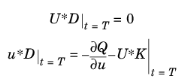
with respect to the control variables ξ evaluated at the final time t=T. The dependent variables, u(ξ), depend on the controls, ξ, but for notational simplicity we will just write u in the following. Note that the objective cannot depend on time derivatives of the dependent variables, that is

(2-14)

This limitation can be circumvented by projecting the time derivative to a dependent variable. The forward solution u is a solution to the parameterized discrete forward problem

(2-15)

where Λ are the constraint Lagrange multipliers, or (generalized) reaction forces, corresponding to the constraints M. It is assumed that Q does not explicitly depend on Λ.

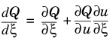
To compute the sensitivity of Q with respect to ξ, first apply the chain rule:

(2-16)

In this expression, the sensitivity of the solution with respect to the control variables, ∂u/∂ξ, is still an unknown quantity. Therefore, differentiate the forward problem, Equation 2-15, formally with respect to ξ:

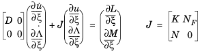
Here, D = −∂L/∂

K = −∂L/∂u, and N = −∂M/∂u as usual. Assuming that the constraint force Jacobian NF is independent of ξ (that is, ∂NF/∂ξ = 0), you can write the above relations in matrix form as

(2-17)

solve for the sensitivities ∂u/∂ξ and ∂Λ/∂ξ, with initial conditions ∂u0/∂ξ and ∂Λ0/∂ξ, respectively, and plug them back for evaluation at t = T into Equation 2-16.

If the number of individual control variables, ξj, is small, Equation 2-17 can be solved for each right-hand side [∂L/∂ξj ∂Μ/∂ξj]T with corresponding initial conditions and the solution inserted into Equation 2-16. This is the forward method, which in addition to the sensitivity dQ/dξ returns the sensitivity of the solution, ∂u/∂ξ. As an alternative, the right-hand side of Equation 2-17 can be calculated by finite differences using the forward numeric method.

If there are many control variables and the sensitivity of the solution itself, ∂u/∂ξ, is not required, the adjoint method is more efficient.

Adjoint Sensitivity

The adjoint sensitivity method is based on using solution variables u* and U* known as the adjoint solution, to rewrite Equation 2-16:

Note that it has been assumed that

The homogeneous adjoint equations are solved backward in time and require “final” conditions for initialization. The final conditions for U* and u* are computed as

On this form, only one forward and one backward (adjoint) problem must be solved regardless of the number of control variables, followed by an evaluation of the gradient for each variable. Obviously, this is much faster than the forward method if the number of variables is large with the drawback that the forward solution must be available at all times during the backward solution of the adjoint. To reduce the memory requirements for this, a checkpointing strategy is employed. This means that at a number of checkpoints the forward solution is stored in memory such that a hot start of the time-dependent solver can be performed to produce the forward solution in higher resolution between checkpoints when needed. This reduces the memory requirement at the cost of one additional forward solution.