The Optimization Solver node () contains settings for selecting a gradient-based optimization method and specifying related solver properties:

The Optimality tolerance, Maximum number of model evaluations, and Method settings are fundamental and can be controlled from an optimization study step.

Choose to let an optimization study step control the fundamental optimization method settings (the default). For User Defined specify the settings directly in this node.

Specify the Optimality tolerance, which has default value 1e-3. See About Gradient-Based Solvers. Note that this can be too strict, in particular if the forward multiphysics model is not solved accurately enough. See About Optimality Tolerances.

Specify the Maximum number of model evaluations, which defaults to 1000. This number limits the number of times the objective function is evaluated, which in most cases is related to the number of times the multiphysics model is simulated for different values of the optimization control variable. Note, however, that it is not equal to the number of iterations taken by the optimizer because each iteration can invoke more than a single objective function evaluation. Furthermore, by setting this parameter to a smaller value and calling the optimization solver repeatedly, you can study the convergence rate and stop when further iterations with the optimization solver no longer have any significant impact on the value of the objective function.

For time-dependent optimization, the objective is evaluated at the final time, but it is possible to let the optimization solver control this time by specifying a Stop expression.

The four available choices are IPOPT (the default), GCMMA, MMA, and Levenberg–Marquardt. The Levenberg–Marquardt method can only be used for problems of least-squares type without constraints, and it is not supported for eigenvalue problems. IPOPT and MMA can solve any type of optimization problem. See About Gradient-Based Solvers.

This setting controls the behavior when the solver node under the Optimization solver node returns a solution containing more than one solution vector (for example, a frequency response). If the gradient step is an eigenvalue study step, the Auto setting correspond to Use first — namely, only the first eigenvalue and eigenfunction are used. The IPOPT and Levenberg–Marquardt solvers, except for the eigenvalue study step, only support the Auto setting, meaning in practice the sum over frequencies and parameters or the last time step. For MMA, the options are as for the derivative-free solvers: Auto, Use first, Use last, Sum of objectives, Minimum of objectives, and Maximum of objectives. The last two settings make the MMA algorithms handle maximin and minimax problems efficiently.

When IPOPT or MMA is used, the expression used as objective function can be controlled through this setting. The default is All, in which case the sum of all objective contributions not deactivated in an optimization study step are used as objective function.

By selecting Manual, you can enter an expression that is used as the objective function in the Objective expression field. The expression all_obj_contrib represents the sum of all objective contributions not deactivated in a controlling optimization study step. Hence, this expressions leads to the same optimization problem as selecting All. Note, however, that MMA treats least-squares objective contributions in a more efficient way when All is selected.

IPOPT, GCMMA/MMA, and Levenberg–Marquardt are gradient-based methods. The gradient can be computed according to the choices Automatic, analytic (the default); Forward; Adjoint; Forward numeric; and Numeric. Moreover, only the Forward and Numeric methods are supported for eigenvalue solvers. When Automatic, analytic is chosen, either the adjoint method or the forward method is used to compute the gradient analytically. The automatically selected method leads to fewer linear solves and thus a lower computational time. The number of linear solves depends on the number of control variables, number of objective functions, and the number of constraints.

It is also possible to explicitly choose to use either the adjoint or forward method using the corresponding alternatives from the menu. With the option Forward numeric, a semianalytic approach is available where the gradient of the PDE residual with respect to control variables is computed by numerical perturbation and then substituted into the forward analytic method. When Numeric is chosen, finite differences are used to compute the gradient numerically.

For time-dependent problems, all analytic gradient methods have options to adjust the default integration tolerances for the sensitivity solver. A separate section titled Transient Adjoint appears, when using the Adjoint gradient method.

For the Forward and Forward numeric gradient methods a Forward sensitivity rtol factor can be specified. This factor multiplied by the forward problem relative tolerance to calculate the relative tolerance for the sensitivity solver. You can also specify a Forward sensitivity scaled atol, which is a global absolute tolerance that is scaled with the initial conditions. The absolute tolerance for the sensitivity solution is updated if scaled absolute tolerances are updated for the forward problem.

When the Numeric gradient method is selected, you can further specify a Difference interval (default 1.5E-8). This is the relative magnitude of the numerical perturbations to use for all numeric differentiation.

You can choose the Gradient approximation order explicitly. Selecting First gives a less accurate gradient, while selecting Second gives a better approximation of the gradient. However, Second requires twice as many evaluations of the objective function for each gradient compared to First. In many applications, the increased accuracy obtained by choosing Second is not worth this extra cost.

The sensitivity of the objective function is by default stored in the solution object such that it can be postprocessed after the solver has completed. To save memory by discarding this information, change Store functional sensitivity to Off. If you instead choose On for results while solving, sensitivity information is also computed continuously during solution and made available for probing and plotting while solving. This is the most expensive option.

Absolute tolerance on the dual infeasibility, see The IPOPT Solver. Successful termination requires that the max-norm of the dual infeasibility is less than the Dual infeasibility absolute tolerance (the default value is 1).

Absolute tolerance on the constraint violation, see The IPOPT Solver. Successful termination requires that the max-norm of the constraint violation is less than the Constraint violation absolute tolerance (The default value is 0.1).

Absolute tolerance on the complementarity, see The IPOPT Solver. Successful termination requires that the max-norm of the complementarity is less than the Complementary conditions absolute tolerance (the default value is 0.1).

You can choose a Linear Solver for the step computations. The options are MUMPS and PARDISO. The default value is MUMPS.

If MUMPS is selected, you can choose Percentage increase in the estimated working space. The default value is 1000. A small value can reduce memory requirements at the expense of computational time.

The Move limits option makes it possible to bound the maximum absolute change for any (scaled) control variable between two outer iterations This is particularly relevant, when MMA is used, because this does not have an inner loop to ensure improvement of the objective and satisfaction of constraints.

By default, the GCMMA and MMA solvers continues to iterate until the relative change in any control variable is less than the optimality tolerance. If the Maximum outer iterations option is enabled, the solver stops either on the tolerance criterion or when the number of iterations is more than the maximum specified.

The GCMMA solver has an inner loop which ensures that each new outer iteration point is feasible and improves on the objective function value. By default, the Maximum number of inner iterations per outer iteration is 10. When the maximum number of inner iterations is reached, the solver continues with the next outer iteration.

The Internal tolerance factor is multiplied by the optimality tolerance to provide an internal tolerance number that is used in the GCMMA/MMA algorithm to determine if the approximations done in the inner loop are feasible and improve on the objective function value. The default is 0.1. Decrease the factor to get stricter tolerances and a more conservative solver behavior.

Both MMA and GCMMA penalize violations of the constraints by a number that is calculated as the specified Constraint penalty factor times 1e-4 divided by the optimality tolerance. Increasing this factor for a given optimality tolerance forces the solver to better respect constraints, while relatively decreasing the influence of the objective function.

By default the solver terminates on the tolerance, but it is possible to terminate prematurely (without triggering a warning) by using setting the Maximum number of outer iterations.

The Levenberg–Marquardt method controls the step length and direction through a positive scalar regularization parameter. A value close to zero means that the optimization solver takes a step close to a full Gauss–Newton step. A large value means that it takes a small step close to the steepest-descent direction. See The Levenberg–Marquardt Solver.

The Levenberg–Marquardt method controls this penalty factor internally and tries to have as small penalty as possible in order to approach second-order Newton convergence. Therefore, a small value of the Initial damping factor means that the solver tries to be aggressive initially, while a large value means that the solver is more cautious.

By default, the Levenberg–Marquardt solver terminates on the controls or the angle between the defect and the Jacobian, but if Terminate also for defect reduction is enabled, the solver will also terminate, if the sum of squares has been reduced by a factor equal to the product of the optimality tolerance and the Defect reduction tolerance factor.

This section only appears, if the Adjoint gradient method is chosen in the Optimization Solver section. You can choose between two solver types:

Unless all forward solutions are stored in memory, the transient adjoint will involve recomputation from the forward solutions that are saved — the checkpoints. This can be avoided by setting Out-of-core for the Forward solution handling. The number of checkpoints is determined the setting for Forward solutions stored between checkpoints:

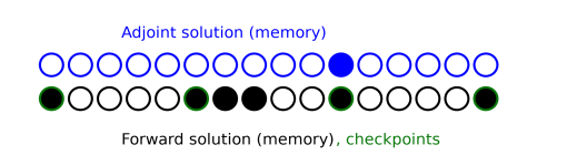
Manual the number of checkpoints is controlled by specifying the maximum number of Forward solutions between checkpoints and in practice this means that the number of checkpoints is identical to the number of steps taken by the solver divided by the number given in this setting. The maximum number of stored forward solutions at anytime will then be the number of checkpoints plus the value given in the setting. Recomputation of the forward solution can thus be avoided by setting a value larger than the number of time steps used for the forward problem, but this also maximizes the memory consumption, see Figure 5-1. Conversely, the memory consumption will be minimized if the number of checkpoints is set to the square root of the number of time steps used for the forward problem.

When Time continuous is chosen, the backward time stepping can be chosen as

The Tolerances of the backward time stepping is determined automatically by default, but it is also possible to manually specify the Adjoint rtol factor and Adjoint scaled atol factors, which control the accuracy of the adjoint solution, similarly to the corresponding Forward sensitivity factors. In addition an Adjoint quadrature rtol factor and an Adjoint quadrature atol can be given. These settings control the relative and absolute accuracy of time integrals (or quadratures) used to calculate objective function gradients. Note that the absolute tolerance is unscaled.

The Keep solutions setting is synchronized from the optimization study step. It is described in The General Optimization Study, see Keep Solutions (Gradient Based).

Select the Plot checkbox to plot the results while solving the model. Select a Plot group from the list and any applicable Probes.

Use the Compensate for nojac terms list to specify whether to try to assemble the complete Jacobian if an incomplete Jacobian has been detected. Select:

From the Adjoint solution choose Initialize with zero solution (the default) or Initialize with forward solution. The latter option can reduce the computational time, if the problem is self-adjoint and an iterative solver is used. This typically happens in linear structural mechanics when the total elastic strain energy variable (Ws_tot) is used as objective. The option only affects the adjoint problem of stationary solvers.

See Theory for Stationary Sensitivity Analysis for details about the algorithm.

In this section you can define constants that can be used as temporary constants in the solver. You can use the constants in the model or to define values for internal solver parameters. Click the Add () button to add a constant and then define its name in the Constant name column and its value (a numerical value or parameter expression) in the Constant value column. By default, any defined parameters are first added as the constant names, but you can change the names to define other constants. Click Delete () to remove the selected constant from the list.

The Log displays the information about the progress of the solver. See The Optimization Solver Log.