Tutorial Model — Topology Optimization
Topology optimization in a structural mechanics context can answer the question: Given that you know the loads on the structure, which distribution of the available material maximizes stiffness? Or, conversely, how much material is necessary to obtain a predefined stiffness, and how should it be distributed? Such investigations typically occur during the concept design stages.
The conflicting goals of stiffness maximization and mass minimization lead to a continuum of possible optimal solutions, depending on how you balance the goals against each other. This topology optimization example demonstrates how to use a penalization method (SIMP) to obtain an optimal distribution of a fixed amount of material such that stiffness is maximized. Changing the amount of material available leads to a different solution that is also Pareto optimal, representing a different balance between the conflicting objectives.
The geometry and load pattern are similar to the Messerschmitt–Bölkow–Blohm beam (MBB) commonly used as a validation test for topology optimization.
Model Definition
The model studies optimal material distribution in the beam, which consists of a linear elastic material, structural steel. The dimensions of the beam region — 6 meters by 1 meter by 0.5 meters — means an original total weight of 23,550 kg. The beam is symmetric about the plane x = 3. Both ends rest on rollers while an edge load acts on the top middle part.
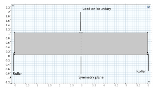
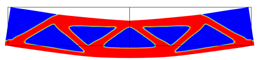
The objective functional for the optimization, which defines the criterion for optimality, is the total strain energy. Note that the strain energy exactly balances the work done by the applied load, so minimizing the strain energy minimizes the displacement induced at the points where load is applied, effectively minimizing the compliance of the structure — maximizing its stiffness. The other, conflicting, objective is minimization of total mass, which is implemented as an upper bound on the mass of the optimized structure.
Another condition that is more difficult to enforce is the requirement that the optimized topology is truly binary — any given point is either solid or void, nothing in between — but still without excessively fine details or “checkerboard” patterns. The SIMP penalization method accomplishes the first part. In the SIMP model, the stress tensor is considered to be a function of the true Young’s modulus E0 and the artificial density, θc, which acts as control variable in the optimization problem:
Since the stiffness must, for numerical reasons, not vanish completely anywhere in the model, the density parameter is constrained such that θmin ≤ ρ ≤ 1. The exponent p ≥ 1 is a penalty factor that makes intermediate densities provide less stiffness compared to what they cost in weight.
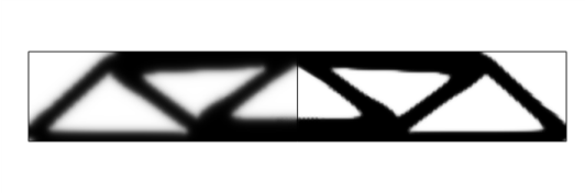
When there is an overall limit on the fraction Vfrac = 0.5 of the domain area, A, occupied by solid material
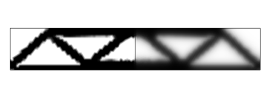
the SIMP penalization forces θc toward either of its bounds. Increasing p therefore leads to a sharper solution.
At the same time, the solution must not contain too much fine details, since that would compromise the reliability of the final design. Also, it is desirable to make the solution as independent of the mesh resolution as possible. To accomplish this, some kind of regularization is needed. There are many possibilities. One of the easiest to implement is based on a combination of successive mesh refinements and minimum length scale imposed via a Helmholtz filter.
The equation essentially just smears out the design as illustrated below with and θc and θf to the left and right, respectively.
The material volume factor (right) has a lot of gray scale.
This filtered design variable can then be projected to reduce the extent of the gray scale region. COMSOL Multiphysics supports projection based on the hyperbolic tangent function (see Ref. 1)
This is illustrated for θβ = 0.5and β = 8 below with θf and θ to the left and right.
The (projected) material volume factor shown to the right has no visible gray scale.
High values of β are associated with strong projection and less gray scale, but also slows down the optimization process, so initially we will not use it and thus set θ = θf.
Results
The following plot shows the stiffness distribution for the optimized solution. The resulting design is an approximation of a truss structure, which is expected for this beam size. Note that the optimal design for a longer or shorter beam may be quite different, and also that there may exist stiffer solutions using the same amount of material. Such solutions typically consist of thinner members that have been eliminated here by the regularization and refinement procedure.
Notes About the COMSOL Implementation
A Solid Mechanics interface represents the structural properties of the beam, while an Optimization interface allows adding the control variable, objective, and constraints for the optimization problem. The total internal strain energy is a predefined variable, solid.Ws_tot, readily available to use as the objective function for the optimization problem.
Only the left half of the beam geometry must be modeled, because of the assumed symmetry, which is implemented as a Roller condition on the symmetry plane. Plots for postprocessing and inspection of the solution while solving are set up using a Mirror dataset, to show the complete solution. The geometry is parameterized, making it easy to experiment with different beam sizes.
The optimization solver is selected and controlled from a Topology Optimization study step. For topology optimization, either the MMA, IPOPT, or the GCMMA solver can be used. They have different merits and weaknesses. MMA and GCMMA tend to be braver in the beginning, proceeding quickly toward an approximate optimum. IPOPT is more cautious, but converges more efficiently close to the final solution due to its second-order approximation of the objective.
This example demonstrates a strategy based on using MMA with a limited number of iterations on successively finer meshes. It quickly and reliably produces trustworthy topologies showing good improvement of the objective function value. These solutions are not necessarily globally optimal, which may, however, be of less importance in practice.