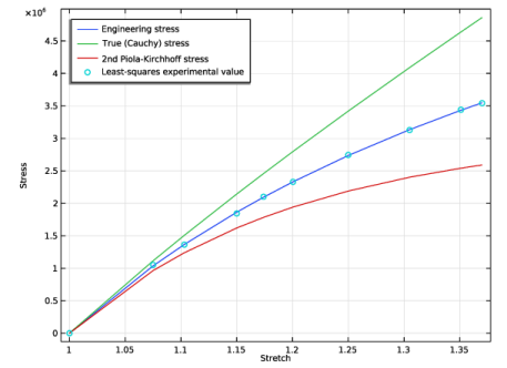
Results
Add a plot of the least-squares fitted stress-strain curve together with the measured data.
1D Plot Group 1
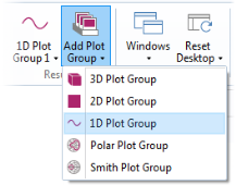
In the Home toolbar, click Add Plot Group
and choose 1D Plot Group
.
Global 1
1
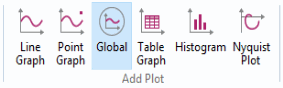
On the 1D plot group toolbar, click Global
.
2
In the Settings window for Global, locate the y-axis data section.
3
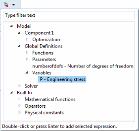
Click Replace Expression
in the upper-right corner of the y-axis data section. From the menu, choose Model > Global Definitions > Variables > P Engineering stress.
4
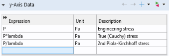
Add two more expressions to plot the true (Cauchy) stress as well as the 2nd Piola–Kirchhoff stress as shown below:stress.
Global 2
1
On the 1D Plot Group 1 toolbar, click Global.
2
In the Settings window for Global, locate the y-axis data section.
3
Click Replace Expression
in the upper-right corner of the y-axis data section. From the menu, choose Model > Solver > Parameter Estimation > opt.glsobj.engStress.data - Least squares experimental value.
4
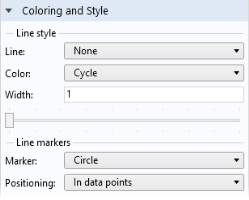
Click to expand the Coloring and style section.
5
Find the Line style subsection. From the Line list, choose None.
6
Find the Line markers subsection. From the Marker list, choose Circle.
7
From the Positioning list, choose In data points.
8
On the 1D plot group toolbar, click Plot
.
Finish the plot by adjusting the title, axis labels, and legend positioning.
9
In the Model Builder click 1D Plot Group 1
.
10
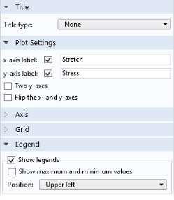
In the Settings window for 1D Plot Group 1 click to expand the Title section. From the Title type list, choose None.
11
Locate the Plot Settings section.
-
Select the x-axis label checkbox.
-
In the
x-axis
label text field, type
Stretch
.
-
Select the y-axis label checkbox.
-
In the y-axis label text field, type
Stress
.
12
Click to expand the Legend section. From the Position list, choose Upper left.
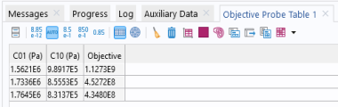
Objective Probe Table 1
You can see the values of the optimized parameters in the last row of the automatically created Objective Probe table.