Examples using the Optimization Module exist in the application library for the Optimization Module, as well as in the Application Libraries for several other modules. Search for optimization in the Application Libraries window search field to find models that use the Optimization Module in the products that your license includes. The models illustrate the use of the Optimization interfaces
It is natural to question how this objective function changes when you vary some parameters or control variables. These variables or parameters can control any part of the design: dimensions, loads, boundary conditions, material properties, material distribution, and so forth. The control variables often have a set of
bounds and
design constraints associated with them: dimensions must be within some limits, geometric features must not come to close to each other, only certain materials are possible, and so on.
When optimizing a system modeled as a Multiphysics model, there may also be performance constraints present, which depend on the model solution. For example, when minimizing the weight of a part, it is often important to keep the maximum stress or temperature below a predefined safety limit.
In general, an optimization problem is when you want to improve the
objective function by varying the
control variables within some set of
constraints. Optimization problems can be further categorized as
topology,
size,
shape, and
parameter optimization.
The Optimization Module contains the framework and functionality needed to perform gradient-based and
gradient-free optimization on an existing COMSOL Multiphysics model.
The plot in Figure 1 shows the hydraulic conductivity obtained by inverse modeling using 24 observations in a model where the aim is to characterize an aquifer. The model is in the Subsurface Flow Module application library and combines the Optimization interface with a Darcy’s Law interface for the fluid flow in the aquifer. The inverse problem in this model is to estimate the hydraulic-conductivity field in the aquifer using experimental data in the form of hydraulic-head measurements from four dipole-pump tests.
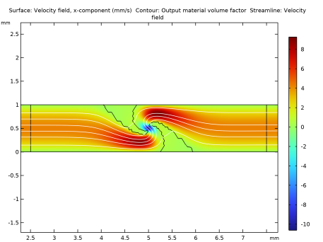
This model is in the Optimization Module Application Library. It combines a Laminar Flow interface for the single-phase flow in the channel and an Optimization interface, where the objective is a scaled x direction velocity that the optimization solver minimizes. The design variable
gamma (
γ) can be interpreted as the local porosity, ranging between 0 (filled) and 1 (open channel), so the contour
γ = 0.5 indicates the border between the open channel and the filling.
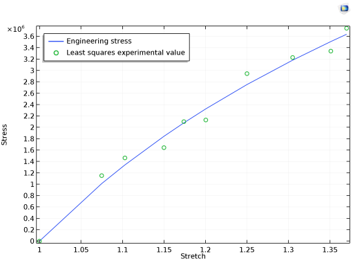
You can use the Optimization Module to perform parameter estimation: to determine input values so that the output matches some experimental data — that is, to solve an inverse problem. The first tutorial (
Tutorial Model — Curve Fitting) describes how to use the Optimization Module for parameter estimation. When solving an inverse problem, there is some set of experimental data that can be compared to the output of the model. Parameter estimation is used to adjust model inputs or properties such that the results agree with the experimental data. Typical objectives include estimating material properties or loads.
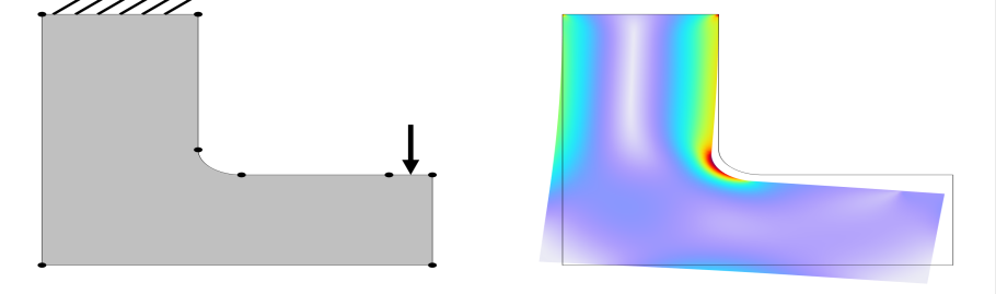
Consider a COMSOL Multiphysics model of a physical system, such as the bracket shown in Figure 4. The part is constrained at the top and loaded on the side. The part must support a known load while staying within acceptable limits on the deflection. However, an experienced structural engineer can quickly recognize that the part is overdesigned. It is possible to remove material from the part, which would reduce the total mass (the cost) of the part, while still staying within the limits on the deflection (the constraints). A closely related problem which is often easier to solve can be stated as: Minimize the compliance (the deflection) of the structure under the condition that the total mass must be reduced by at least some predefined factor.
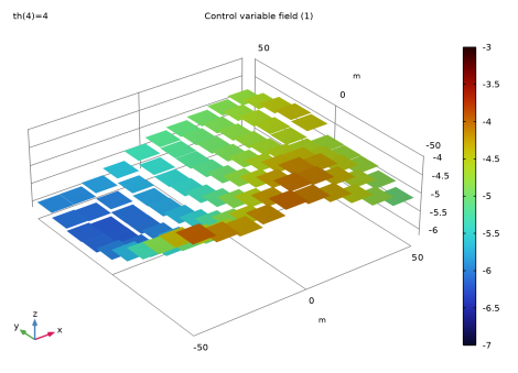
One way to address this is to use topology optimization. Topology optimization treats the material distribution as the design variable. Design variables of this type are treated in the same way as the solution variables; they are interpolated using shape functions on the finite element mesh. Therefore, there is one design variable per mesh node or per mesh element, associated with a position in the geometry. We call this a
control variable field.
The Optimization Module computes the derivative, or the
sensitivity, of the objective function with respect to these discrete design variables. For topology optimization, the
adjoint method is required, because all other methods are too slow. The optimization solver uses the sensitivity information to manipulate the design variables, within the limit of any user-defined constraints, in the direction of improved objective function values.
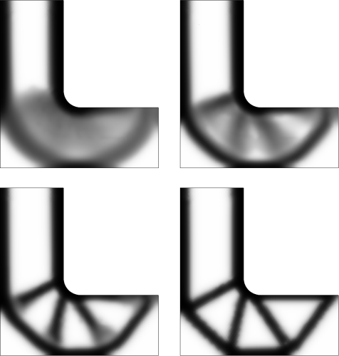
This is an iterative procedure, as illustrated in Figure 5. Starting with the initial design, the solver adjusts the control variables representing a fictitious material density in each element. This is repeated as long as some improvement in the objective function is possible and the constraints are not violated.
Although topology optimization is quick to set up, it has a couple of drawbacks. First, the resulting design does have some dependency on the mesh used. There are techniques known as regularization that you can use to avoid this and the topology model example in this guide includes regularization. Second, it is difficult to incorporate geometric constraints into the optimization algorithm and this can lead to impractical designs, but COMSOL does support the use of milling constraint for topology optimization. This can be used to reduce the design freedom, so that more practical designs are found. In any case, topology optimization should be used early in the design process as a guide for the overall structure of the system. The method becomes more difficult to use efficiently when the design is already quite rigid and only minor modifications to the design are possible. In such situations,
size optimization and
shape optimization become more useful.