The Molecular Flow Module
Vacuum engineers and scientists use the Molecular Flow Module to design vacuum systems and to understand and predict low pressure gas flows. The use of simulation tools in the design cycle has become more widespread as these tools improve understanding, reduce prototyping costs, and speed up development. Vacuum systems are usually very expensive to prototype, consequently increased use of simulation in the design process can result in significant savings.
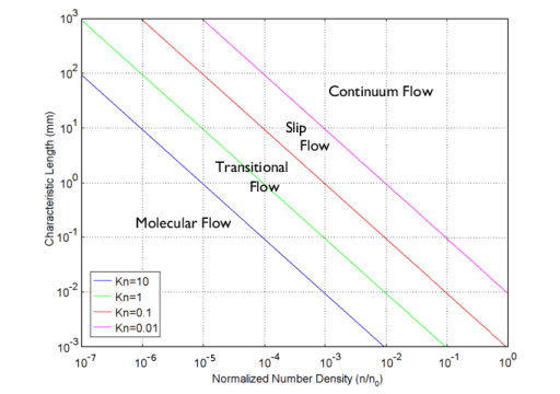
The gas flows that occur inside vacuum systems are described by different physics than conventional fluid flow problems. At low pressures, the mean free path of the gas molecules becomes comparable to the size of the system and gas rarefaction becomes important. The degree of rarefaction is characterized by the Knudsen number, Kn = λ/l, where λ is the mean free path of the gas molecules and l is the characteristic length scale of the system. The Knudsen number increases with decreasing number density (or pressure) and with decreasing system size. As the Knudsen number increases, different flow regimes are encountered, as shown in Figure 1.
Figure 1: Plot showing the main fluid flow regimes for rarefied gas flows. Different regimes are separated by lines of constant Knudsen number. The number density of the gas is normalized to the number density of an ideal gas at atmospheric pressure and a temperature of 0°C (n0).
Knudsen Number Regimes
In the continuum flow regime (Kn < 0.01), the Navier–Stokes equations apply and conventional computational fluid dynamics tools can be used to model the flow.
As the Knudsen number is increased, the slip-flow regime (0.01 < Kn < 0.1) is encountered. The Navier–Stokes equations still apply, but slip boundary conditions must be used at the walls to account for the effect of the Knudsen layer: a thin layer of rarefied gas adjacent to the surfaces of the flow geometry.
At even higher Knudsen numbers, the transitional flow regime (0.1 < Kn < 10) is encountered. The Knudsen layer occupies a significant fraction (or indeed all) of the flow geometry and a kinetic approach must be used to solve the flow.
Finally, at large Knudsen numbers (Kn > 10), molecular flow occurs. In a molecular flow, the gas molecules interact only with the surfaces of the flow domain and there is no scattering between the molecules themselves. The Molecular Flow Module includes predefined physics interfaces, referred to as physics interfaces, which are used to model kinetic gas flows. Both the Free Molecular Flow and the Transitional Flow interfaces are available.
The Free Molecular Flow interface can be used to model nonisothermal free molecular flows inside complex geometries. The physics interface computes the molecular flux on the surfaces of the model. The pressure, number density and heat flux can also be calculated on model surfaces, and the number density can be obtained anywhere interior to the flow domain. The physics interface can model stationary or quasistatic thermal molecular flows. The flow must be quasistatic, as the gas molecules are assumed to travel instantaneously between surfaces in the model. Secondary time-dependent effects, such as the finite time constant for desorption of molecules adsorbed on the surface, can be accounted for in this approach, as the time constants involved are typically much longer than the transit times associated with the molecular velocity and the system size.
Since the gas molecules do not interact with each other in the flow domain, solving for many different species at once does not significantly increase the computational complexity of the problem. It is therefore, quite straightforward to model flows involving several different species simultaneously. Modeling multiple species are required if adsorption and desorption of the molecules occurs, it is also possible for the different species to interact on the surfaces — for example, if they share common adsorption sites the site occupancy can be set up as an expression involving the concentration of both gas molecules.
The Transitional Flow interface can model isothermal molecular or transitional flows across a range of Knudsen numbers. The physics interface uses the discrete velocity method to compute the kinetic flow of gas molecules within the modeling domain. Scattering between the molecules is included in the physics interface (although it can be disabled). Both stationary and time-dependent flows can be modeled.
For any physics interface, a problem is set up by specifying the appropriate boundary and initial conditions in the COMSOL Desktop. COMSOL’s design emphasizes the physics by displaying the equations that are solved by each feature and allowing advanced users full access to change them. There is also great flexibility to add user-defined equations and expressions to the system and to couple together different types of physics. For example, using the Free Molecular Flow interface, you can model heat flow in the walls of a vacuum chamber together with molecular flow just by entering the temperature variable name (computed by the heat transfer system) in the Wall temperature setting. COMSOL Multiphysics automatically performs the coupling when assembling the resulting equation system. The equations are then solved using a range of flexible and powerful solvers. Once a solution is obtained, a wide range of postprocessing tools are available to interpret the data, and predefined plots are automatically generated. COMSOL Multiphysics is very flexible and is able to evaluate a wide range of physical quantities. Predefined quantities include the pressure, number density, molecular flux, and drift velocity (available through easy-to-use menus). Arbitrary user-defined expressions can also be evaluated.
The first step in modeling a vacuum system is typically to define the geometry. The geometry can be imported from a wide range of CAD packages, or dynamically linked to a CAD geometry in third party software using one of the LiveLink products. Alternatively, complex, parameterized geometries can be created within COMSOL Multiphysics from scratch. Next a suitable physics interface is selected and appropriate material properties are added. The initial conditions and boundary conditions are set up in the physics interface and the mesh is defined. In many cases, the suggested mesh, defined from physics-dependent defaults, is appropriate for the problem. A solver is selected (although the physics-dependent default solver is usually appropriate) and the problem is solved. Finally, the results are visualized in the Graphics window, where you can experiment with different plots, animations, and reports to illustrate and describe the model. All of these steps are accessed from the COMSOL Desktop.