PDF

Whispering Gallery Mode Resonator
Introduction
Waves can be confined around the circumference of a structure and exhibit resonant behavior. This principle is valid for different phenomena and length scales showing that underlying concepts can be applied in very different fields - from the 34 m wide Whispering Gallery in the dome of St Paul’s Cathedral, where acoustic waves can travel over large distances, to micrometer sized glass spheres, where light can be confined with extremely low losses due to total reflection. These types of systems are called whispering gallery mode (WGM) resonators.
Figure 1: High order polar mode with radial mode number of l = 2 of a whispering gallery mode (WGM) resonator. The electric field is confined by total internal reflection at the circumference of a glass sphere.
In this model, we calculate the resonance frequency and spatial mode shape of a glass sphere at optical frequencies, also called a microsphere resonator. The approach described here can also be applied to other types of WGM resonators, like toroid, disk, or bottle-type microresonators. These types of devices typically exhibit extremely high optical quality factors (Q factors), a small mode volume, and strong light-material interactions making them useful tools for nonlinear optics, optomechanics, and sensing applications. Because only approximations for the resonance frequency exist, numerical simulations are essential to get insight into device behavior and performance.
To validate the microsphere resonator model and to use it as an initial frequency guess for the numerical simulation, the approximate resonance frequencies are computed based on a series expansion, discussed in Ref. 1, up to a maximum order of kmax = 3.
The highest possible Q factor is often desirable as it typically increases the interaction strength of interest. The Q factor of each mode is limited by several loss channels: material, radiative, and scattering (surface roughness and contamination) (compare with Ref. 2). In this model, no surface roughness or contamination is accounted for, so only material losses Qmat and radiative losses Qrad are contributing. The material losses can be computed from the attenuation coefficient of the material
(1),
where κ is the imaginary part of the complex refractive index N = n  jκ. The Q factor Qmat can be calculated as
(2),
with its corresponding damping
(3).
These parameters give some first insight into the Q-factor limits imposed by finite material losses and will be used in the model definition to find the modes of interest.
Model Definition
To efficiently model such a WGM resonator, a 2D axisymmetric approach is used. The 2D axisymmetric version of the Electromagnetic Waves, Frequency Domain supports a nonzero azimuthal mode number nm such that the electric E field can be written as
(4)
Please note that E is still a three-component vector. The geometry is limited to the area where the modes are located, which helps to reduce the amount of degrees of freedoms in the model. The geometry is surrounded by a Perfectly Matched Layer (PML) to dampen any escaping radiation.
When it comes to meshing, it is advised to manually adjust the mesh for 2D axisymmetric eigenfrequency analysis. The default physics-controlled mesh would mesh the geometry to resolve the wavelength properly. Here, however, the meshing requirement is only that the transverse mode shapes must be properly resolved.
An Eigenfrequency study step is used to compute the field distribution and the respective complex eigenfrequency λ = jω + δ, from which the mode frequency and mode damping δ can be computed. For a resonant structure, you are typically interested in the bound modes in the resonator. It is quite common that unwanted modes, so called spurious modes, exist in the geometry, especially for larger geometries and higher frequencies. This model illustrates two ways, shown in Study 1 and Study 2, to handle these situations efficiently.
Study 1 uses a spatial filtering method. As it is known that a WGM will be located inside the resonator, we can compare the electric field norm inside and outside of the resonator and filter the modes based on a threshold criterion. This is done using two integration operators defining a mode localization variable, ModeLoc, which is used in the Filtering and Sorting section of the Eigenfrequency study settings to remove spurious modes.
Study 2 uses a region in the complex plane to find only the desired eigenmodes. Each mode represents a point in the complex plane. As the losses are dominated by the material absorption in this configuration and we have an estimation of the resonance frequency range, we can use the region search method of the Eigenfrequency study step to find the modes of interest, defined by the real and imaginary part of the eigenvalue λ. The modes of interest will have a small but finite damping, much lower than the spurious modes, which are located outside of the resonator — partly in the absorbing PML.
Study 3 uses a parametric sweep to compute the modes for different resonator radii - demonstrating a configuration of three radial mode numbers, l, and two polarizations (TE and TM). The azimuthal mode number nm is adjusted to keep the resonance wavelength around 1 μm
Results and Discussion
Figure 2 shows the Q factor of all modes in the model in addition to the mode localization. For a mode localization of 1, the field norm is completely located within the resonator domain. The modes with a low Q factor and a low mode localization number are strongly damped and located outside the resonator and are, thus, not modes of interest. This information can be used to filter the modes, which is done in Study 1.
Figure 2: Q factor and mode localization of computed modes, gray dashed lines show the mode frequencies.
Figure 3 shows the damping of the modes computed in Study 1 and the modes found by the region search in Study 2. The region search is set up such that only modes with a damping lower than the threshold are searched for. The frequency and damping of the modes of interest are identical although different methods are used to find them.
Figure 3: Blue points correspond to the damping of the modes found in Study 1. The back line is the upper limit for the damping (imaginary part of the eigenvalue) in the region search. Therefore, only modes with a lower damping are found in study 2 (green circles).
Figure 4 shows that for large radii, the Q factor is limited by the material loss (dashed line). For a small radius of r = 10 μm, radiative losses become the dominant loss factor, leading to a further reduction of the Q factor.
Figure 4: Q factor for different modes and radii. The solid black line corresponds to the Q-factor limit by the material absorption.
Figure 5 shows the tracked modes of the resonator for different radii.
.
Figure 5: Frequencies of a selection of whispering gallery modes for different resonator sizes.
Figure 6 shows a 3D representation of the resonator mode using the Revolution 2D dataset.
Figure 6: Reconstructed mode from the 2D axisymmetric solution. The electric field direction is represented by red arrows, the surface plots show the electric field norm while the contour plot illustrates the .
References
1. S. Schiller, “Asymptotic expansion of morphological resonance frequencies in Mie scattering,” Appl. Opt., vol. 32, pp. 2181–2185, 1993.
2. M. Gorodetsky, A. Savchenkov, and V. Ilchenko, “Ultimate Q of optical microsphere resonators,” Opt. Lett., vol. 21, pp. 453–455, 1996.
Application Library path: Wave_Optics_Module/Verification_Examples/whispering_gallery_mode_resonator
Modeling Instructions
From the File menu, choose New.
New
In the New window, click  Model Wizard.
Model Wizard
1
In the Model Wizard window, click  2D Axisymmetric.
2
In the Select Physics tree, select Optics > Wave Optics > Electromagnetic Waves, Frequency Domain (ewfd).
3
Click Add.
4
Click  Study.
5
In the Select Study tree, select General Studies > Eigenfrequency.
6
Global Definitions
Resonator Parameters
1
In the Model Builder window, under Global Definitions click Parameters 1.
2
In the Settings window for Parameters, type Resonator Parameters in the Label text field.
3
Locate the Parameters section. Click  Load from File.
4
Browse to the model’s Application Libraries folder and double-click the file whispering_gallery_mode_resonator_resonator_parameters.txt.
Analytic Higher Order Approximation - Schiller
1
In the Home toolbar, click  Parameters and choose Add > Parameters.
2
In the Settings window for Parameters, type Analytic Higher Order Approximation - Schiller in the Label text field.
3
Locate the Parameters section. Click  Load from File.
4
Browse to the model’s Application Libraries folder and double-click the file whispering_gallery_mode_resonator_analytic_higher_order_approximation_parameters.txt.
Airy Function Zeroes
1
In the Home toolbar, click  Functions and choose Global > Interpolation.
2
In the Settings window for Interpolation, type Airy Function Zeroes in the Label text field.
3
Locate the Definition section. In the Function name text field, type Ai.
4
Click  Load from File.
5
Browse to the model’s Application Libraries folder and double-click the file whispering_gallery_mode_resonator_airy_function_zeroes.txt.
Piecewise 1 (pw1)
1
In the Home toolbar, click  Functions and choose Global > Piecewise.
2
In the Settings window for Piecewise, type dk in the Function name text field.
3
Locate the Definition section. Find the Intervals subsection. Click  Load from File.
4
Browse to the model’s Application Libraries folder and double-click the file whispering_gallery_mode_resonator_piecewise_function.txt.
Geometry 1
1
In the Model Builder window, under Component 1 (comp1) click Geometry 1.
2
In the Settings window for Geometry, locate the Units section.
3
From the Length unit list, choose µm.
Rectangle 1 (r1)
1
In the Geometry toolbar, click  Rectangle.
2
In the Settings window for Rectangle, locate the Size and Shape section.
3
In the Width text field, type r_air-r_cut.
4
In the Height text field, type h_air.
5
Locate the Position section. In the r text field, type r_cut.
6
In the z text field, type -h_air/2.
7
Click to expand the Layers section. In the table, enter the following settings:
8
Select the Layers to the right checkbox.
9
Select the Layers on top checkbox.
10
Click  Build Selected.
Circle 1 (c1)
1
In the Geometry toolbar, click  Circle.
2
In the Settings window for Circle, locate the Size and Shape section.
3
In the Radius text field, type r_res.
4
Locate the Rotation Angle section. In the Rotation text field, type 45.
5
Click  Build Selected.
6
Click the  Zoom Extents button in the Graphics toolbar.
Union 1 (uni1)
1
In the Geometry toolbar, click  Booleans and Partitions and choose Union.
2
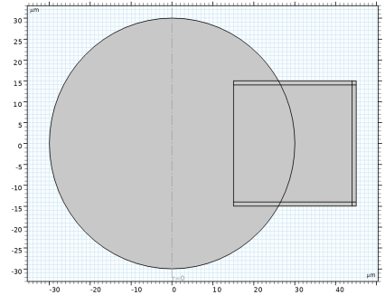
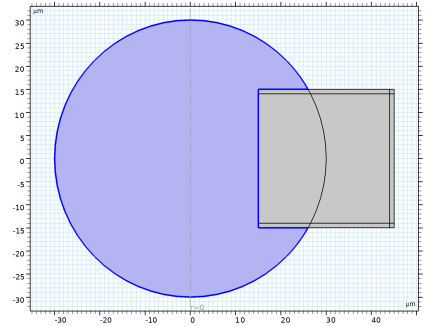
Click in the Graphics window and then press Ctrl+A to select both objects. Alternatively, you can left-click on the circle and the rectangle to add them to the Union selection.
3
In the Settings window for Union, click  Build Selected.
Delete Entities 1 (del1)
1
In the Geometry toolbar, click  Delete.
2
In the Settings window for Delete Entities, locate the Entities or Objects to Delete section.
3
From the Geometric entity level list, choose Domain.
4
On the object uni1, select Domain 1 only.
5
Click  Build All Objects.
6
Click the  Zoom Extents button in the Graphics toolbar.
Partition Edges 1 (pare1)
In order to have more control over the mesh, we can partition the outer edge to later refine the mesh close to where the mode will be located.
1
In the Geometry toolbar, click  Booleans and Partitions and choose Partition Edges.
2
On the object del1, select Boundary 24 only.
3
In the Settings window for Partition Edges, locate the Positions section.
4
5
In the Geometry toolbar, click  Build All.
Materials
Host Medium
1
In the Model Builder window, under Component 1 (comp1) right-click Materials and choose Blank Material.
2
In the Settings window for Material, type Host Medium in the Label text field.
3
Locate the Material Contents section. In the table, enter the following settings:
Sphere
1
Right-click Materials and choose Blank Material.
2
In the Settings window for Material, type Sphere in the Label text field.
3
4
Locate the Material Contents section. In the table, enter the following settings:
Electromagnetic Waves, Frequency Domain (ewfd)
1
In the Model Builder window, under Component 1 (comp1) click Electromagnetic Waves, Frequency Domain (ewfd).
2
In the Settings window for Electromagnetic Waves, Frequency Domain, locate the Out-of-Plane Wave Number section.
3
In the m text field, type n_m.
Definitions
Integration 1 (intop1)
1
In the Definitions toolbar, click  Nonlocal Couplings and choose Integration.
2
In the Settings window for Integration, type res in the Operator name text field.
3
Integration 2 (intop2)
1
In the Definitions toolbar, click  Nonlocal Couplings and choose Integration.
2
In the Settings window for Integration, type air in the Operator name text field.
3
Variables 1
1
In the Model Builder window, right-click Definitions and choose Variables.
2
In the Settings window for Variables, locate the Variables section.
3
This globally available variable will be used to filter the modes based on their location.
Perfectly Matched Layer 1 (pml1)
1
In the Definitions toolbar, click  Perfectly Matched Layer.
2
3
In the Settings window for Perfectly Matched Layer, locate the Geometry section.
4
From the Type list, choose Cylindrical.
Mesh 1
1
In the Model Builder window, under Component 1 (comp1) click Mesh 1.
2
In the Settings window for Mesh, locate the Sequence Type section.
3
From the list, choose User-controlled mesh.
Size
1
In the Model Builder window, under Component 1 (comp1) > Mesh 1 click Size.
2
In the Settings window for Size, locate the Element Size Parameters section.
3
In the Maximum element size text field, type 1.25.
4
In the Minimum element size text field, type 0.1.
Size 1
1
In the Model Builder window, click Size 1.
2
In the Settings window for Size, locate the Element Size Parameters section.
3
In the Maximum element size text field, type 1.
4
In the Minimum element size text field, type 0.009.
5
Select the Maximum element growth rate checkbox. In the associated text field, type 1.04.
Size 2
Now, add another size node to refine the mesh at the outer boundary. This will help resolve the mode shape in the resonator and the exponential decay of the field in the air domain.
1
In the Model Builder window, right-click Mesh 1 and choose Size.
2
Drag and drop Size 2 below Size 1.
3
In the Settings window for Size, locate the Geometric Entity Selection section.
4
From the Geometric entity level list, choose Boundary.
5
6
Locate the Element Size section. Click the Custom button.
7
Locate the Element Size Parameters section.
8
Select the Maximum element size checkbox. In the associated text field, type 0.15.
9
Click  Build All.
Filtered Eigenfrequency Study
This first study will demonstrate how to use the Filtering setting in the Eigenfrequency study to filter out unwanted, nonbound, modes.
1
In the Model Builder window, click Study 1.
2
In the Settings window for Study, type Filtered Eigenfrequency Study in the Label text field.
Step 1: Eigenfrequency
1
In the Model Builder window, under Filtered Eigenfrequency Study click Step 1: Eigenfrequency.
2
In the Settings window for Eigenfrequency, locate the Study Settings section.
3
Select the Desired number of eigenfrequencies checkbox. In the associated text field, type 200.
4
In the Search for eigenfrequencies around shift text field, type f_res.
5
Click to expand the Filtering and Sorting section. Find the Filtering subsection. In the table, enter the following settings:
This filters the modes in the solution based on the localization using a threshold value.
6
In the Study toolbar, click  Compute.
Results
Electric Field - Filtered Modes
In the Settings window for 2D Plot Group, type Electric Field - Filtered Modes in the Label text field.
Surface 1
1
In the Model Builder window, expand the Electric Field - Filtered Modes node, then click Surface 1.
2
In the Settings window for Surface, locate the Coloring and Style section.
3
From the Color table list, choose AuroraBorealis.
Arrow Surface 1
1
In the Model Builder window, right-click Electric Field - Filtered Modes and choose Arrow Surface.
2
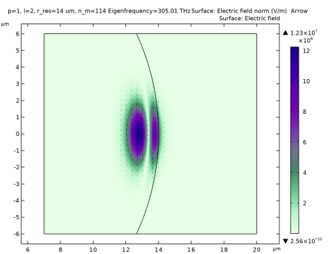
In the Settings window for Arrow Surface, click Replace Expression in the upper-right corner of the Expression section. From the menu, choose Component 1 (comp1) > Electromagnetic Waves, Frequency Domain > Electric > ewfd.Er,ewfd.Ez - Electric field.
3
Locate the Arrow Positioning section. Find the R grid points subsection. In the Points text field, type 40.
4
Find the Z grid points subsection. In the Points text field, type 40.
5
Locate the Coloring and Style section. From the Arrow length list, choose Logarithmic.
6
From the Color list, choose Black.
7
In the Electric Field - Filtered Modes toolbar, click  Plot.
This plot shows the lowest order whispering gallery mode, for the selected azimuthal mode number. The arrow plot indicates that the field is polarized in the z direction.
Mode Localization
1
In the Results toolbar, click  1D Plot Group.
2
In the Settings window for 1D Plot Group, type Mode Localization in the Label text field.
3
Locate the Plot Settings section. Select the Two y-axes checkbox.
4
Locate the Axis section. Select the Secondary y-axis log scale checkbox.
5
Click to expand the Legend section. From the Position list, choose Lower left.
Add a line segment plot to show where the data points align with the found frequencies.
Line Segments 1
1
In the Mode Localization toolbar, click  Line Segments.
2
In the Settings window for Line Segments, locate the x-Coordinates section.
3
4
Locate the y-Coordinates section. In the table, enter the following settings:
5
Click to expand the Coloring and Style section. Find the Line style subsection. From the Line list, choose Dashed.
6
From the Color list, choose Gray.
Mode Localization
In the Mode Localization toolbar, click  Global.
Global 1
1
In the Settings window for Global, locate the y-Axis Data section.
2
3
Locate the x-Axis Data section. From the Parameter list, choose Expression.
4
In the Expression text field, type ewfd.freq.
5
From the Unit list, choose THz.
6
Click to expand the Coloring and Style section. Find the Line style subsection. From the Line list, choose None.
7
Find the Line markers subsection. From the Marker list, choose Circle.
Mode Localization
In the Model Builder window, click Mode Localization.
Global 2
1
In the Mode Localization toolbar, click  Global.
2
In the Settings window for Global, locate the y-Axis section.
3
Select the Plot on secondary y-axis checkbox.
4
Locate the y-Axis Data section. In the table, enter the following settings:
5
Locate the x-Axis Data section. From the Parameter list, choose Expression.
6
In the Expression text field, type ewfd.freq.
7
From the Unit list, choose THz.
8
Locate the Coloring and Style section. Find the Line style subsection. From the Line list, choose None.
9
Find the Line markers subsection. From the Marker list, choose Point.
Mode Localization
1
In the Model Builder window, click Mode Localization.
2
In the Settings window for 1D Plot Group, locate the Grid section.
3
Clear the Show grid checkbox.
4
In the Mode Localization toolbar, click  Plot.
This plot shows that a model localization factor of 0.5 can be efficiently used to discriminate between the whispering gallery modes that have a large Q factor as only resonator modes with a localization factor over 0.94 are found. To see the unwanted modes localized in the surrounding air with a low Q factor, the study can be rerun without filtering.
Add Study
The second study will demonstrate how to use the Region method in the Eigenfrequency solver to filter out unwanted, nonbound, modes.
1
In the Home toolbar, click  Add Study to open the Add Study window.
2
Go to the Add Study window.
3
Find the Studies subsection. In the Select Study tree, select General Studies > Eigenfrequency.
4
Click the Add Study button in the window toolbar.
5
In the Home toolbar, click  Add Study to close the Add Study window.
Eigenfrequency Region Search
In the Settings window for Study, type Eigenfrequency Region Search in the Label text field.
Step 1: Eigenfrequency
1
In the Model Builder window, under Eigenfrequency Region Search click Step 1: Eigenfrequency.
2
In the Settings window for Eigenfrequency, locate the Study Settings section.
3
From the Eigenfrequency search method list, choose Rectangle.
4
In the Approximate number of eigenfrequencies text field, type 100.
5
Find the Rectangle search region subsection. In the Smallest real part (Eigenfrequency) text field, type f_res-5[THz].
6
In the Largest real part (Eigenfrequency) text field, type f_res+20[THz].
7
In the Largest imaginary part (Eigenfrequency) text field, type (damp+500[kHz])/(2*pi).
8
In the Study toolbar, click  Compute.
Results
Electric Field - Region Search
1
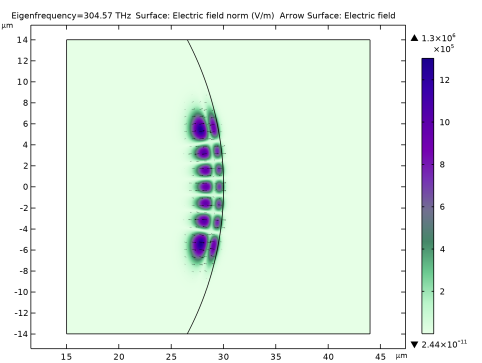
In the Settings window for 2D Plot Group, type Electric Field - Region Search in the Label text field.
2
Locate the Data section. From the Eigenfrequency (THz) list, choose 299.29.
Surface 1
1
In the Model Builder window, expand the Electric Field - Region Search node, then click Surface 1.
2
In the Settings window for Surface, locate the Coloring and Style section.
3
From the Color table list, choose AuroraBorealis.
Arrow Surface 1
Now, we can copy the Arrow Surface plot we created earlier.
In the Model Builder window, under Results > Electric Field - Filtered Modes right-click Arrow Surface 1 and choose Copy.
Arrow Surface 1
1
In the Model Builder window, right-click Electric Field - Region Search and choose Paste Arrow Surface.
2
In the Electric Field - Region Search toolbar, click  Plot.
3
In the Model Builder window, click Arrow Surface 1.
It is clear from these plots that the eigenfrequency region search method only returns the wanted whispering gallery modes.
Filter Criterion
To show the filtered mode spectrum, we can create a new 1D plot group.
1
In the Results toolbar, click  1D Plot Group.
2
In the Settings window for 1D Plot Group, type Filter Criterion in the Label text field.
3
Locate the Plot Settings section. Clear the Two y-axes checkbox.
4
Locate the Axis section. Select the y-axis log scale checkbox.
5
Locate the Legend section. From the Position list, choose Upper right.
Global 1
In the Filter Criterion toolbar, click  Global.
Filtered Modes
1
In the Model Builder window, expand the Results > Filter Criterion node, then click Global 1.
2
In the Settings window for Global, type Filtered Modes in the Label text field.
3
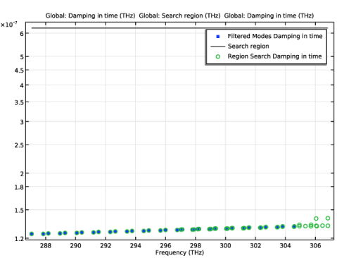
Click Replace Expression in the upper-right corner of the y-Axis Data section. From the menu, choose Component 1 (comp1) > Electromagnetic Waves, Frequency Domain > ewfd.damp - Damping in time - Hz.
4
Locate the y-Axis Data section. In the table, enter the following settings:
5
Locate the x-Axis Data section. From the Parameter list, choose Expression.
6
In the Expression text field, type freq.
7
From the Unit list, choose THz.
8
Locate the Coloring and Style section. Find the Line style subsection. From the Line list, choose None.
9
Find the Line markers subsection. From the Marker list, choose Point.
10
Click to expand the Legends section. Find the Include subsection. Select the Label checkbox.
Filter Criterion
In the Filter Criterion toolbar, click  Global.
Global 2
1
In the Settings window for Global, locate the Data section.
2
From the Dataset list, choose Eigenfrequency Region Search/Solution 2 (sol2).
Now, add a line to show the search region expression, ewfd.Qfactor, for reference.
3
Locate the y-Axis Data section. In the table, enter the following settings:
4
Locate the x-Axis Data section. From the Parameter list, choose Expression.
5
In the Expression text field, type freq.
6
From the Unit list, choose THz.
7
Locate the Coloring and Style section. From the Color list, choose Black.
Region Search
1
In the Model Builder window, right-click Filtered Modes and choose Duplicate.
2
In the Settings window for Global, type Region Search in the Label text field.
3
Locate the Data section. From the Dataset list, choose Eigenfrequency Region Search/Solution 2 (sol2).
4
Locate the Coloring and Style section. Find the Line markers subsection. From the Marker list, choose Circle.
5
Click to expand the Legends section. Find the Include subsection. Select the Label checkbox.
6
In the Filter Criterion toolbar, click  Plot.
This plot indicates that the damping can be used with the eigenfrequency region search method, to discriminate between the whispering gallery modes and the modes located in the surrounding air. The solid line shows the threshold value. It is clear that the whispering gallery modes from both the first study (blue circles) and second study (green circles) fall below this threshold value.
Add Study
In the final, third, study, parametric sweeps will be used together with the Eigenfrequency solver to show the solutions for some resonator configurations.
1
In the Home toolbar, click  Add Study to open the Add Study window.
2
Go to the Add Study window.
3
Find the Studies subsection. In the Select Study tree, select General Studies > Eigenfrequency.
4
Click the Add Study button in the window toolbar.
5
In the Home toolbar, click  Add Study to close the Add Study window.
Parametric Sweep Eigenfrequency Study
In the Settings window for Study, type Parametric Sweep Eigenfrequency Study in the Label text field.
Step 1: Eigenfrequency
1
In the Model Builder window, under Parametric Sweep Eigenfrequency Study click Step 1: Eigenfrequency.
2
In the Settings window for Eigenfrequency, locate the Study Settings section.
3
Select the Desired number of eigenfrequencies checkbox. In the associated text field, type 1.
4
In the Search for eigenfrequencies around shift text field, type f_res.
Parametric Sweep
1
In the Study toolbar, click  Parametric Sweep.
2
In the Settings window for Parametric Sweep, locate the Study Settings section.
3
4
5
6
Parametric Sweep 2
1
In the Study toolbar, click  Parametric Sweep.
2
In the Settings window for Parametric Sweep, locate the Study Settings section.
3
From the Sweep type list, choose All combinations.
4
5
6
7
8
In the Study toolbar, click  Compute.
Results
Electric Field - Different Configurations
1
In the Settings window for 2D Plot Group, type Electric Field - Different Configurations in the Label text field.
2
Locate the Data section. From the Parameter value (p,l) list, choose 2: p=1, l=2.
3
From the Parameter value (r_res (um),n_m) list, choose 2: r_res=14 um, n_m=114.
Surface 1
1
In the Model Builder window, expand the Electric Field - Different Configurations node, then click Surface 1.
2
In the Settings window for Surface, locate the Coloring and Style section.
3
From the Color table list, choose AuroraBorealis.
Arrow Surface 1
In the Model Builder window, under Results > Electric Field - Region Search right-click Arrow Surface 1 and choose Copy.
Arrow Surface 1
1
In the Model Builder window, right-click Electric Field - Different Configurations and choose Paste Arrow Surface.
2
Click the  Zoom Extents button in the Graphics toolbar.
3
In the Electric Field - Different Configurations toolbar, click  Plot.
4
In the Model Builder window, click Arrow Surface 1.
In this plot group, you can visualize the whispering gallery modes for some resonator configurations.
3D Sector
Next, use the available revolution dataset to make a 3D visualization of the modes.
1
In the Results toolbar, click  3D Plot Group.
2
In the Settings window for 3D Plot Group, type 3D Sector in the Label text field.
3
Locate the Data section. From the Dataset list, choose Revolution 2D 3.
4
From the Parameter value (p,l) list, choose 3: p=1, l=3.
5
From the Parameter value (r_res (um),n_m) list, choose 1: r_res=10 um, n_m=80.
Multislice 1
1
In the 3D Sector toolbar, click  More Plots and choose Multislice.
2
In the Settings window for Multislice, locate the Multiplane Data section.
3
Find the X-planes subsection. In the Planes text field, type 0.
4
Find the Y-planes subsection. In the Planes text field, type 0.
5
Locate the Coloring and Style section. From the Color table list, choose AuroraBorealis.
Revolution 2D 3
1
In the Model Builder window, expand the Results > Datasets node, then click Revolution 2D 3.
2
In the Settings window for Revolution 2D, click to expand the Revolution Layers section.
3
From the Number of layers list, choose Custom.
4
In the Layers text field, type 100.
5
In the Start angle text field, type -105.
6
In the Revolution angle text field, type 15.
Arrow Volume 1
1
In the Model Builder window, right-click 3D Sector and choose Arrow Volume.
2
In the Settings window for Arrow Volume, locate the Expression section.
3
In the R-component text field, type ewfd.Er*exp(-i*n_m*rev3phi).
4
In the PHI-component text field, type ewfd.Ephi*exp(-i*n_m*rev3phi).
5
In the Z-component text field, type ewfd.Ez*exp(-i*n_m*rev3phi).
6
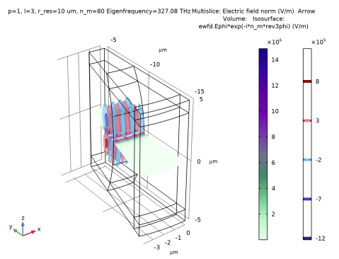
Locate the Arrow Positioning section. Find the X grid points subsection. In the Points text field, type 100.
7
Find the Y grid points subsection. In the Points text field, type 100.
8
Find the Z grid points subsection. In the Points text field, type 1.
Isosurface 1
1
Right-click 3D Sector and choose Isosurface.
2
In the Settings window for Isosurface, locate the Expression section.
3
In the Expression text field, type ewfd.Ephi*exp(-i*n_m*rev3phi).
4
Locate the Levels section. From the Entry method list, choose Levels.
5
In the Levels text field, type range(-1.2e6,0.5e6,1.2e6).
6
Locate the Coloring and Style section. From the Color table list, choose Wave.
7
From the Scale list, choose Linear symmetric.
Transparency 1
1
Right-click Isosurface 1 and choose Transparency.
2
In the Settings window for Transparency, locate the Transparency section.
3
Find the Transparency subsection. In the Transparency text field, type 0.45.
4
In the 3D Sector toolbar, click  Plot.
Quality Factor for Different Modes and Radii
1
In the Results toolbar, click  1D Plot Group.
2
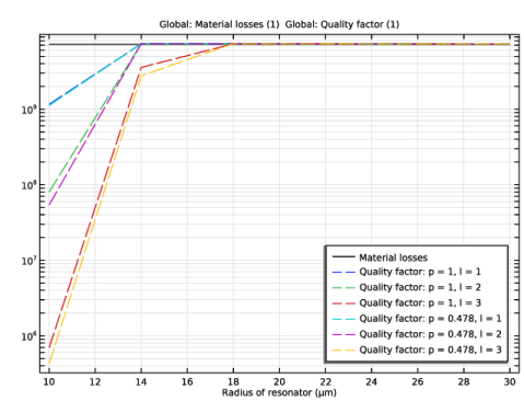
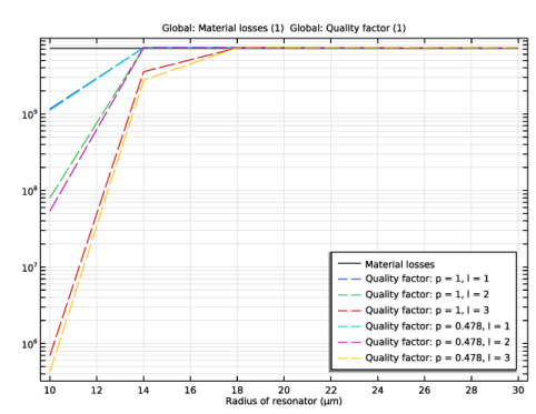
In the Settings window for 1D Plot Group, type Quality Factor for Different Modes and Radii in the Label text field.
3
Locate the Data section. From the Dataset list, choose Parametric Sweep Eigenfrequency Study/Parametric Solutions 1 (sol4).
4
Locate the Plot Settings section. Clear the Two y-axes checkbox.
5
Locate the Axis section. Select the y-axis log scale checkbox.
6
Locate the Legend section. From the Position list, choose Lower right.
Global 1
1
In the Quality Factor for Different Modes and Radii toolbar, click  Global.
First, add the baseline material losses, Q_mat.
2
In the Settings window for Global, locate the y-Axis Data section.
3
4
Locate the x-Axis Data section. From the Axis source data list, choose All solutions.
5
From the Parameter list, choose Expression.
6
In the Expression text field, type r_res.
7
Locate the Coloring and Style section. From the Color list, choose Black.
8
Find the Line markers subsection. From the Marker list, choose None.
Quality Factor for Different Modes and Radii
In the Quality Factor for Different Modes and Radii toolbar, click  Global.
Global 2
1
In the Settings window for Global, locate the Data section.
2
From the Dataset list, choose Parametric Sweep Eigenfrequency Study/Parametric Solutions 1 (sol4).
3
From the Parameter selection (p, l) list, choose From list.
4
In the Parameter values (p,l) list box, select 1: p=1, l=1.
5
Locate the y-Axis Data section. In the table, enter the following settings:
6
Locate the x-Axis Data section. From the Axis source data list, choose All solutions.
7
From the Parameter list, choose Expression.
8
In the Expression text field, type r_res.
9
Locate the Coloring and Style section. Find the Line style subsection. From the Line list, choose Dashed.
10
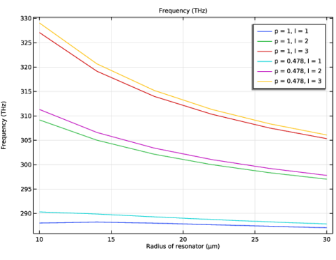
Click to expand the Legends section. Find the Prefix and suffix subsection. In the Suffix text field, type : p = eval(p), l = eval(l).
Global 3
1
Right-click Results > Quality Factor for Different Modes and Radii > Global 2 and choose Duplicate.
2
In the Settings window for Global, locate the Data section.
3
In the Parameter values (p,l) list box, select 2: p=1, l=2.
4
Click to expand the Title section. From the Title type list, choose None.
Global 4
1
Right-click Global 3 and choose Duplicate.
2
In the Settings window for Global, locate the Data section.
3
In the Parameter values (p,l) list box, select 3: p=1, l=3.
Global 5
1
Right-click Global 4 and choose Duplicate.
2
In the Settings window for Global, locate the Data section.
3
In the Parameter values (p,l) list box, select 4: p=0.47846, l=1.
Global 6
1
Right-click Global 5 and choose Duplicate.
2
In the Settings window for Global, locate the Data section.
3
In the Parameter values (p,l) list box, select 5: p=0.47846, l=2.
Global 7
1
Right-click Global 6 and choose Duplicate.
2
In the Settings window for Global, locate the Data section.
3
In the Parameter values (p,l) list box, select 6: p=0.47846, l=3.
4
In the Quality Factor for Different Modes and Radii toolbar, click  Plot.
This plot demonstrates that for large resonator radii, the losses are limited by the material loss, whereas for small radii, radiation loss dominates.
Frequency - Different Modes and Radii
1
In the Results toolbar, click  1D Plot Group.
2
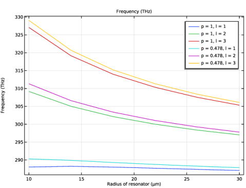
In the Settings window for 1D Plot Group, type Frequency - Different Modes and Radii in the Label text field.
Global 1
1
In the Frequency - Different Modes and Radii toolbar, click  Global.
2
In the Settings window for Global, locate the Data section.
3
From the Dataset list, choose Parametric Sweep Eigenfrequency Study/Parametric Solutions 1 (sol4).
4
From the Parameter selection (p, l) list, choose From list.
5
In the Parameter values (p,l) list box, select 1: p=1, l=1.
6
Locate the y-Axis Data section. In the table, enter the following settings:
7
Locate the x-Axis Data section. From the Axis source data list, choose Outer solutions.
8
From the Parameter list, choose Expression.
9
In the Expression text field, type r_res.
10
Click to expand the Legends section. From the Legends list, choose Evaluated.
11
In the Legend text field, type p = eval(p), l = eval(l).
Global 2
1
Right-click Global 1 and choose Duplicate.
2
In the Settings window for Global, locate the Data section.
3
In the Parameter values (p,l) list box, select 2: p=1, l=2.
4
Click to expand the Title section. From the Title type list, choose None.
Global 3
1
Right-click Global 2 and choose Duplicate.
2
In the Settings window for Global, locate the Data section.
3
In the Parameter values (p,l) list box, select 3: p=1, l=3.
Global 4
1
Right-click Global 3 and choose Duplicate.
2
In the Settings window for Global, locate the Data section.
3
In the Parameter values (p,l) list box, select 4: p=0.47846, l=1.
Global 5
1
Right-click Global 4 and choose Duplicate.
2
In the Settings window for Global, locate the Data section.
3
In the Parameter values (p,l) list box, select 5: p=0.47846, l=2.
Global 6
1
Right-click Global 5 and choose Duplicate.
2
In the Settings window for Global, locate the Data section.
3
In the Parameter values (p,l) list box, select 6: p=0.47846, l=3.
4
In the Frequency - Different Modes and Radii toolbar, click  Plot.
This plot demonstrates the TE and TM modes (p = 1 and p = 0.478) for different radial orders (l).
Eigenfrequencies (ewfd)
Finally, update the expressions in the global evaluations in the evaluation groups to extract numerical values for the results.
1
In the Model Builder window, expand the Results > Eigenfrequencies (ewfd) node, then click Eigenfrequencies (ewfd).
2
In the Settings window for Global Evaluation, locate the Expressions section.
3
4
In the Eigenfrequencies (ewfd) toolbar, click  Evaluate.
Eigenfrequencies (ewfd)
1
In the Model Builder window, expand the Results > Eigenfrequencies (ewfd) 1 node, then click Eigenfrequencies (ewfd).
2
In the Settings window for Global Evaluation, locate the Expressions section.
3
4
In the Eigenfrequencies (ewfd) 1 toolbar, click  Evaluate.