PDF

Single-Bit Hologram
Introduction
A hologram is a holographically recorded object. When two coherent light beams intersect each other, an interference pattern is generated. If this occurs in a material that is sensitive to light intensities greater than a certain exposure threshold, the interference pattern is recorded in the material as a modulation of the refractive index. Such a material is called a holographic material and the process of recording is called holographic recording. When one of the two light beams is originally scattered by an object before entering the holographic material, the beam is called the object beam while the other beam is called the reference beam. In this case, the recorded hologram also contains the information about the scattering object. Now, if the hologram is illuminated by the reference beam alone in the same optical setup, the object beam will be regenerated from the holographic material. This process is called the holographic retrieval. This concept is depicted in Figure 1.
Figure 1: Holographic recording and retrieval.
Model Definition
In this model, the simplest example is chosen, in which the object beam has the same profile as the reference beam. The reference beam enters a holographic material from the left boundary while the object beam enters it from the top boundary. In the recording process, the two beams cross at 90 degree angle in the material and make interference fringes tilted at 45 degrees. For intensities above a certain exposure threshold, a refractive index modulation is induced in the holographic material on top of the constant background refractive index. In the retrieval, only the reference beam illuminates the hologram. Then this beam is partially transmitted and partially reflected off by the hologram, which regenerates the object beam. You can say that the hologram is working as a volume Bragg grating satisfying the Bragg condition for the reference beam.
Results and Discussion
Figure 2 shows the electric field distribution during the recording phase. Notice that the intensity pattern in the rightmost figure shows diagonal stripes that result in the striped refractive index modulation, shown in Figure 3.
Figure 2: Electric field distribution during recording. The left figure show the z-component of the electric field, whereas the right figure shows the squared norm of the electric field.
Figure 3: The refractive index distribution.
Figure 4 shows the intensity distribution across a cross section of the beam. The red line indicates the exposure threshold level for the holographic material. Notice that the refractive index modulation in Figure 5 starts at the location where the threshold level intersects the intensity distribution. In the wings of the beam, the intensity level is too low to induce any refractive index modulation.
Figure 4: The electric field distribution during recording. The blue curve shows the squared electric field norm, whereas the red line indicates the exposure threshold for the holographic material.
Figure 5: The induced refractive index modulation.
Finally, Figure 6 shows the electric field distribution during the retrieval phase. Here, only the reference beam is incident. However, as it is scattered by the induced refractive index grating, the object beam is regenerated and propagates toward the bottom of the figure.
Figure 6: The electric field distribution during the retrieval phase. The left figure shows the z-component of the electric field, whereas the right figure shows the norm of the electric field.
Application Library path: Wave_Optics_Module/Gratings_and_Metamaterials/single_bit_hologram
Modeling Instructions
From the File menu, choose New.
New
In the New window, click  Model Wizard.
Model Wizard
1
In the Model Wizard window, click  2D.
2
In the Select Physics tree, select Optics > Wave Optics > Electromagnetic Waves, Frequency Domain (ewfd).
3
Click Add.
4
Click  Study.
5
In the Select Study tree, select Preset Studies for Selected Physics Interfaces > Wavelength Domain.
6
Global Definitions
Start by loading the parameters that defines the model geometry and material properties.
Parameters 1
1
In the Model Builder window, under Global Definitions click Parameters 1.
2
In the Settings window for Parameters, locate the Parameters section.
3
Click  Load from File.
4
Geometry 1
The simulation domain consists of a rectangle with width L and height H.
1
In the Model Builder window, under Component 1 (comp1) click Geometry 1.
2
In the Settings window for Geometry, locate the Units section.
3
From the Length unit list, choose µm.
Rectangle 1 (r1)
1
In the Geometry toolbar, click  Rectangle.
2
In the Settings window for Rectangle, locate the Size and Shape section.
3
In the Width text field, type L.
4
In the Height text field, type H.
5
Locate the Position section. From the Base list, choose Center.
6
Click  Build All Objects.
Materials
Material 1 (mat1)
1
In the Model Builder window, under Component 1 (comp1) right-click Materials and choose Blank Material.
2
In the Settings window for Material, locate the Material Contents section.
3
Definitions
A maximum operator will be used later when defining the refractive index variation of the hologram.
Maximum 1 (maxop1)
1
In the Definitions toolbar, click  Nonlocal Couplings and choose Maximum.
2
Refractive Index During Recording
Now, define the refractive indices that will be used for the recording phase and the retrieval phase. This variable will later define the refractive index for the material. In the study steps, you later define which of the two refractive index variables that will be used for the different phases.
1
In the Model Builder window, right-click Definitions and choose Variables.
2
In the Settings window for Variables, type Refractive Index During Recording in the Label text field.
3
Locate the Variables section. In the table, enter the following settings:
Modulated Refractive Index
1
Right-click Refractive Index During Recording and choose Duplicate.
2
In the Settings window for Variables, type Modulated Refractive Index in the Label text field.
3
Locate the Variables section. In the table, enter the following settings:
Refractive Index During Retrieval
1
In the Model Builder window, right-click Definitions and choose Variables.
2
In the Settings window for Variables, type Refractive Index During Retrieval in the Label text field.
3
Locate the Variables section. In the table, enter the following settings:
The withsol operator allows you to use expressions from a previous solution. In this case, it is the solution from the first study step, here denoted sol2, that will be used for defining the refractive index distribution during the second study step.
Materials
Material 1 (mat1)
1
In the Model Builder window, under Component 1 (comp1) > Materials click Material 1 (mat1).
2
In the Settings window for Material, locate the Material Contents section.
3
Electromagnetic Waves, Frequency Domain (ewfd)
As the same study will include both the study step for the recording of the hologram and the study step for the retrieval of the object beam, all features required for both study steps will be added to the physics in the next step. Later on, the physics trees will be modified in the study step settings.
1
In the Model Builder window, under Component 1 (comp1) click Electromagnetic Waves, Frequency Domain (ewfd).
2
In the Settings window for Electromagnetic Waves, Frequency Domain, locate the Components section.
3
From the Electric field components solved for list, choose Out-of-plane vector.
Reference Scattering Boundary Condition
1
In the Physics toolbar, click  Boundaries and choose Scattering Boundary Condition.
2
In the Settings window for Scattering Boundary Condition, type Reference Scattering Boundary Condition in the Label text field.
3
4
Locate the Scattering Boundary Condition section. From the Incident field list, choose Wave given by E field.
5
Specify the E0 vector as
This defines the input electric field for the reference beam.
Object Scattering Boundary Condition
1
In the Physics toolbar, click  Boundaries and choose Scattering Boundary Condition.
2
In the Settings window for Scattering Boundary Condition, type Object Scattering Boundary Condition in the Label text field.
3
4
Locate the Scattering Boundary Condition section. From the Incident field list, choose Wave given by E field.
5
Specify the E0 vector as
Recording Scattering Boundary Condition
1
In the Physics toolbar, click  Boundaries and choose Scattering Boundary Condition.
2
In the Settings window for Scattering Boundary Condition, type Recording Scattering Boundary Condition in the Label text field.
3
Retrieval Scattering Boundary Condition
1
Right-click Recording Scattering Boundary Condition and choose Duplicate.
2
In the Settings window for Scattering Boundary Condition, type Retrieval Scattering Boundary Condition in the Label text field.
3
Mesh 1
Free Triangular 1
Set the maximum mesh element size to be one tenth of the material wavelength.
In the Mesh toolbar, click  Free Triangular.
Size
1
In the Model Builder window, click Size.
2
In the Settings window for Size, locate the Element Size section.
3
Click the Custom button.
4
Locate the Element Size Parameters section. In the Maximum element size text field, type wl0/n1/10.
Study 1
Now, define the two study steps.
Recording
1
In the Model Builder window, under Study 1 click Step 1: Wavelength Domain.
2
In the Settings window for Wavelength Domain, type Recording in the Label text field.
3
Locate the Study Settings section. In the Wavelengths text field, type wl0.
4
Locate the Physics and Variables Selection section. Select the Modify model configuration for study step checkbox.
5
In the tree, select Component 1 (comp1) > Definitions > Refractive Index During Retrieval.
6
7
In the tree, select Component 1 (comp1) > Electromagnetic Waves, Frequency Domain (ewfd) > Retrieval Scattering Boundary Condition.
8
Retrieval
1
Right-click Study 1 > Step 1: Recording and choose Duplicate.
2
In the Settings window for Wavelength Domain, type Retrieval in the Label text field.
3
Locate the Physics and Variables Selection section. In the tree, select Component 1 (comp1) > Definitions > Refractive Index During Recording.
4
5
In the tree, select Component 1 (comp1) > Definitions > Refractive Index During Retrieval.
6
7
In the tree, select Component 1 (comp1) > Electromagnetic Waves, Frequency Domain (ewfd) > Recording Scattering Boundary Condition.
8
9
In the tree, select Component 1 (comp1) > Electromagnetic Waves, Frequency Domain (ewfd) > Retrieval Scattering Boundary Condition.
10
Solution 1 (sol1)
Before clicking Compute, add a Solution Store, after the node Stationary Solver 1, to store the solution from the first study step.
1
In the Study toolbar, click  Show Default Solver.
Move the node Solution Store 1 to be located between Stationary Solver 1 and Compile Equations: Retrieval.
2
Right-click Solution 1 (sol1) and choose Other > Solution Store.
3
In the Study toolbar, click  Compute.
Results
Recording
Modify the default plot to show the interference between the reference beam and the object beam, by displaying the electric field and the square of the norm of the electric field.
1
In the Settings window for 2D Plot Group, locate the Data section.
2
From the Dataset list, choose Study 1/Solution Store 1 (sol2). This selects the dataset for the first study step.
3
In the Label text field, type Recording.
Surface 1
1
In the Model Builder window, expand the Recording node, then click Surface 1.
2
In the Settings window for Surface, locate the Expression section.
3
In the Expression text field, type ewfd.Ez.
4
Locate the Coloring and Style section. Clear the Color legend checkbox.
Surface 2
1
Right-click Results > Recording > Surface 1 and choose Duplicate.
2
In the Settings window for Surface, locate the Expression section.
3
In the Expression text field, type ewfd.normE^2.
Transformation 1
1
Right-click Surface 2 and choose Transformation.
2
In the Settings window for Transformation, locate the Transformation section.
3
In the X text field, type 34.
Recording
1
In the Model Builder window, under Results click Recording.
2
In the Settings window for 2D Plot Group, click to expand the Title section.
3
From the Title type list, choose Manual.
4
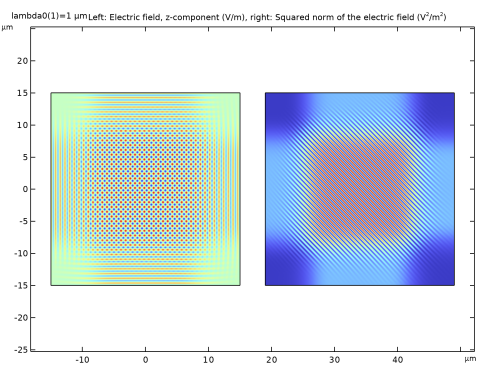
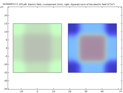
In the Title text area, type Left: Electric field, z-component (V/m), right: Squared norm of the electric field (V<sup>2</sup>/m<sup>2</sup>).
5
In the Recording toolbar, click  Plot.
6
Click the  Zoom Extents button in the Graphics toolbar.
Now, duplicate this plot group to create a plot of the modulated refractive index.
Recording 1
Right-click Recording and choose Duplicate.
Surface 2
1
In the Model Builder window, expand the Recording 1 node.
2
Right-click Surface 2 and choose Delete.
Modulated Refractive Index
1
In the Model Builder window, under Results click Recording 1.
2
In the Settings window for 2D Plot Group, type Modulated Refractive Index in the Label text field.
3
Locate the Title section. In the Title text area, type Modulated refractive index.
Surface 1
1
In the Model Builder window, click Surface 1.
2
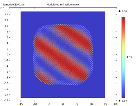
In the Settings window for Surface, click Replace Expression in the upper-right corner of the Expression section. From the menu, choose Component 1 (comp1) > Definitions > Variables > n_mod - Modulated refractive index.
3
Locate the Coloring and Style section. Select the Color legend checkbox.
Modulated Refractive Index
1
In the Model Builder window, click Modulated Refractive Index.
2
In the Settings window for 2D Plot Group, locate the Color Legend section.
3
Select the Show maximum and minimum values checkbox.
4
In the Modulated Refractive Index toolbar, click  Plot.
5
Click the  Zoom Extents button in the Graphics toolbar.
Cut Line 2D 1
1
In the Results toolbar, click  Cut Line 2D.
2
In the Settings window for Cut Line 2D, locate the Data section.
3
From the Dataset list, choose Study 1/Solution Store 1 (sol2).
4
Locate the Line Data section. In row Point 1, set X to -L/2.
5
In row Point 1, set Y to -H/2.
6
In row Point 2, set X to L/2.
7
In row Point 2, set Y to H/2.
Squared Norm of the Electric Field
1
In the Results toolbar, click  1D Plot Group.
2
In the Settings window for 1D Plot Group, type Squared Norm of the Electric Field in the Label text field.
3
Locate the Data section. From the Dataset list, choose Cut Line 2D 1.
Line Graph 1
1
Right-click Squared Norm of the Electric Field and choose Line Graph.
2
In the Settings window for Line Graph, locate the y-Axis Data section.
3
In the Expression text field, type ewfd.normE^2.
4
Click to expand the Legends section. Select the Show legends checkbox.
5
From the Legends list, choose Manual.
6
Line Graph 2
1
Right-click Line Graph 1 and choose Duplicate.
2
In the Settings window for Line Graph, locate the y-Axis Data section.
3
In the Expression text field, type threshold*maxop1(ewfd.normE^2).
4
Click to expand the Coloring and Style section. From the Color list, choose Red.
5
From the Width list, choose 4.
6
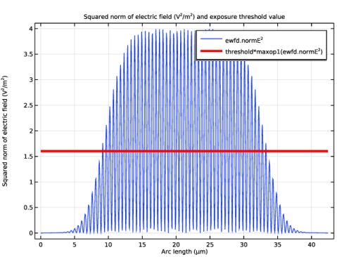
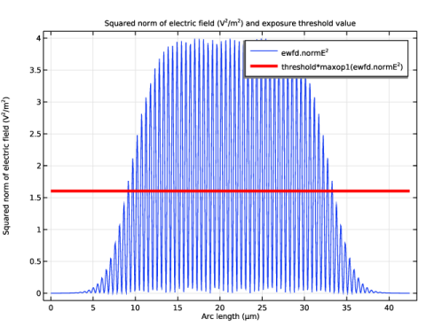
Locate the Legends section. In the table, enter the following settings:
Squared Norm of the Electric Field
1
In the Model Builder window, click Squared Norm of the Electric Field.
2
In the Settings window for 1D Plot Group, click to expand the Title section.
3
From the Title type list, choose Manual.
4
In the Title text area, type Squared norm of electric field (V<sup>2</sup>/m<sup>2</sup>) and exposure threshold value.
5
Locate the Plot Settings section.
6
Select the y-axis label checkbox. In the associated text field, type Squared norm of electric field (V<sup>2</sup>/m<sup>2</sup>).
7
In the Squared Norm of the Electric Field toolbar, click  Plot.
Modulated Refractive Index Line Plot
1
In the Results toolbar, click  1D Plot Group.
2
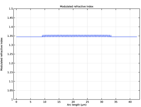
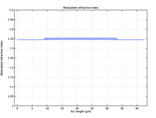
In the Settings window for 1D Plot Group, type Modulated Refractive Index Line Plot in the Label text field.
3
Locate the Data section. From the Dataset list, choose Cut Line 2D 1.
Line Graph 1
1
Right-click Modulated Refractive Index Line Plot and choose Line Graph.
2
In the Settings window for Line Graph, click Replace Expression in the upper-right corner of the y-Axis Data section. From the menu, choose Component 1 (comp1) > Definitions > Variables > n_mod - Modulated refractive index.
Modulated Refractive Index Line Plot
1
In the Model Builder window, click Modulated Refractive Index Line Plot.
2
In the Settings window for 1D Plot Group, locate the Axis section.
3
Select the Manual axis limits checkbox.
4
In the y minimum text field, type 1.
5
In the y maximum text field, type 1.5.
6
In the Modulated Refractive Index Line Plot toolbar, click  Plot.
Retrieval (Reference Only)
1
In the Model Builder window, right-click Recording and choose Duplicate.
2
In the Settings window for 2D Plot Group, type Retrieval (Reference Only) in the Label text field.
3
Locate the Data section. From the Dataset list, choose Study 1/Solution 1 (sol1).
4
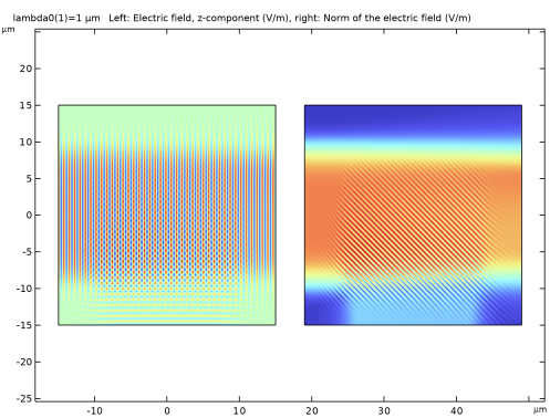
Locate the Title section. In the Title text area, type Left: Electric field, z-component (V/m), right: Norm of the electric field (V/m).
Surface 2
1
In the Model Builder window, expand the Retrieval (Reference Only) node, then click Surface 2.
2
In the Settings window for Surface, locate the Expression section.
3
In the Expression text field, type ewfd.normE.
4
In the Retrieval (Reference Only) toolbar, click  Plot.
5
Click the  Zoom Extents button in the Graphics toolbar.