| 
|
|
|
|


|
1
|
|
2
|
|
3
|
Click Add.
|
|
4
|
Click
|
|
5
|
|
6
|
Click
|
|
1
|
|
2
|
|
3
|
|
1
|
|
2
|
|
3
|
|
4
|
Browse to the model’s Application Libraries folder and double-click the file sesam_laser_heating_sesam_parameters.txt.
|
|
1
|
|
2
|
|
3
|
|
4
|
Browse to the model’s Application Libraries folder and double-click the file sesam_laser_heating_beam_parameters.txt.
|
|
1
|
|
2
|
|
3
|
|
4
|
|
5
|
|
6
|
|
1
|
|
2
|
|
3
|
|
4
|
|
5
|
|
1
|
|
2
|
|
3
|
On the object r2, select Domain 1 only.
|
|
1
|
|
2
|
|
3
|
|
4
|
|
5
|
|
6
|
|
1
|
|
2
|
|
3
|
On the object r3, select Domain 1 only.
|
|
1
|
|
2
|
|
3
|
|
4
|
|
5
|
|
1
|
|
2
|
|
3
|
|
4
|
|
5
|
|
6
|
|
1
|
|
2
|
|
3
|
On the object r4, select Domain 1 only.
|
|
1
|
|
2
|
|
3
|
|
4
|
Click
|
|
1
|
|
2
|
|
3
|
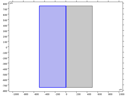
On the object uni1, select Domain 63 only.
|
|
1
|
|
2
|
|
3
|
|
4
|
|
5
|
Click OK.
|
|
1
|
|
2
|
|
3
|
|
4
|
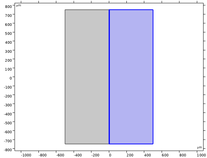
On the object uni1, select Boundary 4 only.
|
|
1
|
In the Model Builder window, under Component 1 (comp1) click Electromagnetic Waves, Beam Envelopes (ewbe).
|
|
3
|
|
4
|
|
1
|
|
2
|
|
4
|
In the Settings window for Scattering Boundary Condition, locate the Scattering Boundary Condition section.
|
|
5
|
|
6
|
|
7
|
|
8
|
|
9
|
|
1
|
|
1
|
|
1
|
|
2
|
Go to the Add Physics window.
|
|
3
|
|
4
|
Click the Add to Component 1 button in the window toolbar.
|
|
5
|
|
1
|
|
2
|
|
1
|
|
2
|
|
1
|
|
2
|
|
3
|
From the list, choose User-controlled mesh.
|
|
4
|
|
1
|
|
3
|
|
4
|
|
1
|
|
3
|
|
4
|
|
1
|
|
2
|
|
1
|
|
3
|
|
4
|
|
5
|
|
6
|
|
7
|
|
1
|
|
2
|
|
3
|
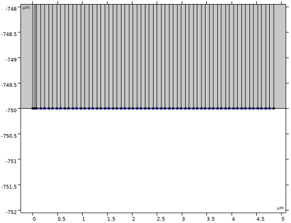
Select the Adjust edge mesh checkbox.
|
|
4
|
Click
|
|
1
|
|
2
|
|
3
|
|
4
|
Locate the Variables section. In the table, enter the following settings:
|
|
1
|
|
2
|
|
3
|
Locate the Variables section. In the table, enter the following settings:
|
|
1
|
|
2
|
|
3
|
|
4
|
|
1
|
|
2
|
|
3
|
|
1
|
|
2
|
|
3
|
|
4
|
|
1
|
|
2
|
|
3
|
|
1
|
|
2
|
Go to the Add Material window.
|
|
3
|
|
4
|
Click the Add to Component button in the window toolbar.
|
|
5
|
In the tree, select Optical > Inorganic Materials > As - Arsenides > Models and simulations > GaAs (Gallium arsenide) (Adachi 1989: n,k 0.207-12.4 um).
|
|
6
|
Click the Add to Component button in the window toolbar.
|
|
1
|
|
2
|
|
3
|
Locate the Material Contents section. In the table, enter the following settings:
|
|
1
|
Go to the Add Material window.
|
|
2
|
In the tree, select Optical > Inorganic Materials > As - Arsenides > Models and simulations > AlAs (Aluminium arsenide) (Rakic and Majewski 1996: n,k 0.221-2.48 um).
|
|
3
|
Click the Add to Component button in the window toolbar.
|
|
1
|
|
2
|
|
3
|
Locate the Material Contents section. In the table, enter the following settings:
|
|
1
|
Go to the Add Material window.
|
|
2
|
In the tree, select Optical > Miscellaneous > Semiconductor alloys > GaAs-InAs (Gallium indium arsenide, GaInAs) (Adachi 1989: n,k 0.207-12.4 um).
|
|
3
|
Click the Add to Component button in the window toolbar.
|
|
4
|
|
1
|
|
2
|
|
3
|
Locate the Material Contents section. In the table, enter the following settings:
|
|
1
|
|
2
|
|
3
|
Click
|
|
1
|
|
2
|
|
3
|
|
1
|
|
2
|
|
3
|
Click
|
|
1
|
|
2
|
Drag and drop below Parametric Sweep.
|
|
3
|
|
4
|
In the Solve for column of the table, under Component 1 (comp1), clear the checkboxes for Solid Mechanics (solid) and Moving Mesh.
|
|
5
|
|
1
|
|
2
|
|
3
|
In the Model Builder window, expand the Study 1 > Solver Configurations > Solution 1 (sol1) > Stationary Solver 2 node.
|
|
4
|
Right-click Study 1 > Solver Configurations > Solution 1 (sol1) > Stationary Solver 2 and choose Segregated.
|
|
5
|
In the Model Builder window, expand the Study 1 > Solver Configurations > Solution 1 (sol1) > Stationary Solver 2 > Segregated 1 node, then click Segregated Step.
|
|
6
|
|
7
|
In the Variables list, choose Spatial Mesh Displacement (comp1.spatial.disp), Temperature (comp1.T), and Displacement Field (comp1.u).
|
|
8
|
|
9
|
In the Model Builder window, under Study 1 > Solver Configurations > Solution 1 (sol1) > Stationary Solver 2 right-click Segregated 1 and choose Segregated Step.
|
|
10
|
|
11
|
|
12
|
In the Add dialog, in the Variables list, choose Spatial Mesh Displacement (comp1.spatial.disp), Temperature (comp1.T), and Displacement Field (comp1.u).
|
|
13
|
Click OK.
|
|
14
|
|
1
|
|
2
|
|
3
|
|
4
|
|
5
|
|
6
|
Click
|
|
1
|
In the Model Builder window, under Results > Datasets right-click Study 1/Parametric Solutions 1 (sol3) and choose Duplicate.
|
|
2
|
|
3
|
|
1
|
|
2
|
|
3
|
|
4
|
|
5
|
|
6
|
|
7
|
|
8
|
Click
|
|
1
|
|
2
|
|
3
|
|
4
|
Locate the Expressions section. In the table, enter the following settings:
|
|
5
|
Click
|
|
1
|
|
1
|
|
1
|
|
2
|
|
1
|
|
2
|
|
3
|
|
4
|
|
1
|
|
1
|
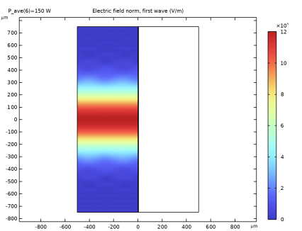
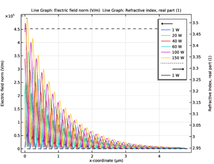
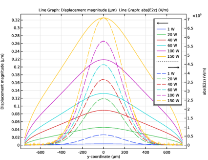
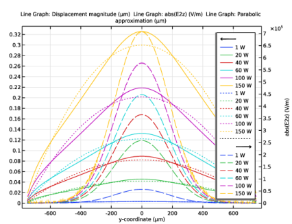
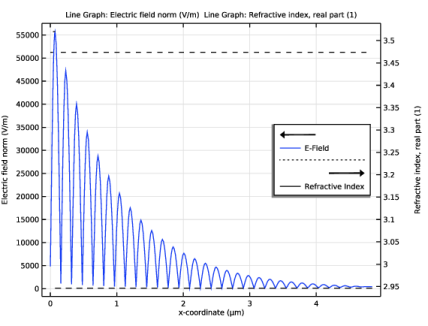
In the Model Builder window, expand the Results > Electric Field, Second Wave (ewbe) node, then click Electric Field.
|
|
2
|
|
3
|
|
4
|
|
1
|
|
2
|
|
3
|
|
4
|
|
1
|
|
2
|
|
3
|
Select the Show legends checkbox.
|
|
4
|
|
5
|
|
1
|
|
2
|
|
3
|
|
4
|
|
5
|
|
6
|
|
7
|
|
1
|
|
2
|
|
3
|
|
4
|
|
1
|
|
2
|
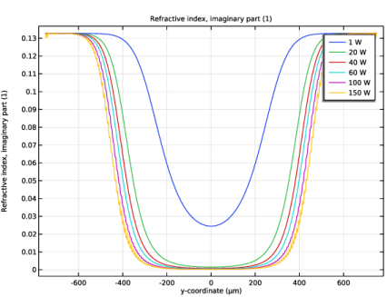
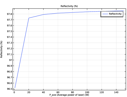
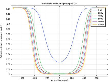
In the Settings window for 1D Plot Group, type Absorption in QW, y Direction in the Label text field.
|
|
3
|
|
1
|
|
2
|
|
3
|
|
4
|
|
5
|
|
6
|
|
7
|
|
1
|
|
2
|
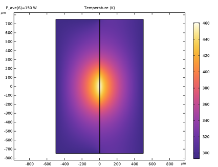
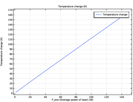
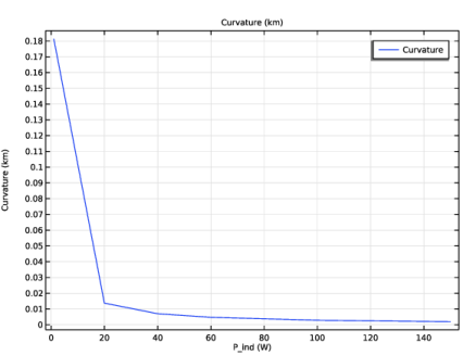
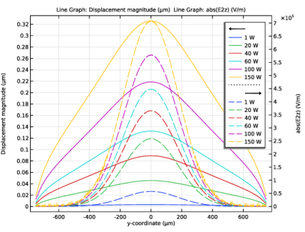
In the Settings window for 1D Plot Group, type Temperature with Laser Power in the Label text field.
|
|
3
|
|
1
|
|
2
|
|
4
|
|
1
|
|
2
|
|
3
|
|
4
|
|
1
|
|
2
|
|
4
|
|
1
|
|
2
|
|
3
|
|
4
|
|
5
|
|
1
|
|
2
|
|
3
|
|
4
|
|
5
|
|
6
|
|
7
|
|
1
|
|
2
|
|
3
|
|
4
|
|
5
|
|
6
|
|
7
|
|
8
|
|
9
|
|
10
|
|
1
|
|
2
|
Go to the Add Physics window.
|
|
3
|
|
4
|
Click the Add to Component 1 button in the window toolbar.
|
|
5
|
|
1
|
|
3
|
|
4
|
|
5
|
|
6
|
Click OK.
|
|
7
|
|
8
|
Click
|
|
9
|
In the Source term quantity table, enter the following settings:
|
|
1
|
|
2
|
|
3
|
In the Solve for column of the table, under Component 1 (comp1), clear the checkbox for Global ODEs and DAEs (ge).
|
|
1
|
|
2
|
In the Settings window for Frequency–Stationary, locate the Physics and Variables Selection section.
|
|
3
|
In the Solve for column of the table, under Component 1 (comp1), clear the checkbox for Global ODEs and DAEs (ge).
|
|
1
|
|
2
|
Go to the Add Study window.
|
|
3
|
Find the Studies subsection. In the Select Study tree, select Preset Studies for Some Physics Interfaces > Stationary.
|
|
4
|
Click the Add Study button in the window toolbar.
|
|
5
|
|
1
|
|
2
|
Clear the Generate default plots checkbox.
|
|
1
|
|
2
|
|
3
|
Click
|
|
1
|
|
2
|
|
3
|
In the Solve for column of the table, under Component 1 (comp1), clear the checkboxes for Solid Mechanics (solid) and Heat Transfer in Solids (ht).
|
|
4
|
In the Solve for column of the table, under Component 1 (comp1) > Multiphysics, clear the checkboxes for Electromagnetic Heating 1 (emh1) and Thermal Expansion 1 (te1).
|
|
5
|
In the Solve for column of the table, under Component 1 (comp1), clear the checkbox for Moving Mesh.
|
|
1
|
In the Model Builder window, expand the Study 2 > Solver Configurations > Solution 10 (sol10) > Stationary Solver 1 node, then click Fully Coupled 1.
|
|
2
|
|
3
|
|
4
|
|
1
|
|
1
|
|
2
|
|
3
|
|
4
|
|
5
|
|
6
|
|
7
|
|
8
|
|
9
|
|
10
|
|
11
|
|
1
|
|
2
|
|
3
|
|
1
|
|
2
|
|
3
|
Click
|
|
5
|