|
|
|

|
1
|
|
2
|
In the Select Physics tree, select Optics > Wave Optics > Electromagnetic Waves, Frequency Domain (ewfd).
|
|
3
|
Click Add.
|
|
4
|
Click
|
|
5
|
In the Select Study tree, select Preset Studies for Selected Physics Interfaces > Wavelength Domain.
|
|
6
|
Click
|
|
1
|
|
2
|
|
1
|
|
2
|
|
3
|
|
4
|
Click to expand the Layers section. In the table, enter the following settings:
|
|
5
|
Click
|
|
6
|
|
7
|
|
8
|
|
9
|
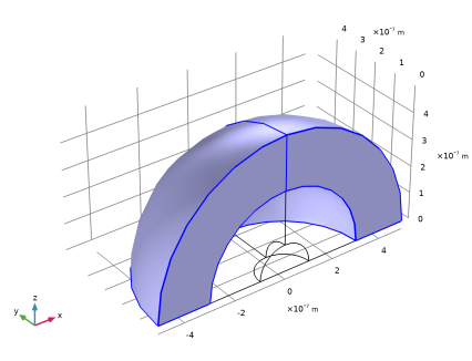
Select the xy-plane: remove z<0 checkbox.
|
|
10
|
Select the zx-plane: remove y<0 checkbox.
|
|
11
|
|
12
|
|
1
|
|
2
|
|
1
|
|
2
|
|
1
|
|
2
|
Go to the Add Material window.
|
|
3
|
|
4
|
Click the Add to Component button in the window toolbar.
|
|
5
|
In the tree, select Optical > Inorganic Materials > Au - Gold > Models and simulations > Au (Gold) (Rakic et al. 1998: Brendel-Bormann model; n,k 0.248-6.20 um).
|
|
6
|
Click the Add to Component button in the window toolbar.
|
|
7
|
|
1
|
In the Model Builder window, under Component 1 (comp1) click Electromagnetic Waves, Frequency Domain (ewfd).
|
|
2
|
|
3
|
From the list, choose Scattered field.
|
|
4
|
|
1
|
|
1
|
|
3
|
|
4
|
|
1
|
|
2
|
|
4
|
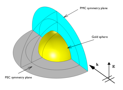
Locate the Symmetry Plane section. From the Symmetry type list, choose Zero tangential electric field (PEC).
|
|
1
|
|
2
|
|
1
|
In the Model Builder window, expand the Far-Field Domain 1 node, then click Far-Field Calculation 1.
|
|
2
|
|
3
|
|
1
|
|
3
|
|
4
|
|
1
|
|
2
|
|
3
|
|
4
|
|
5
|
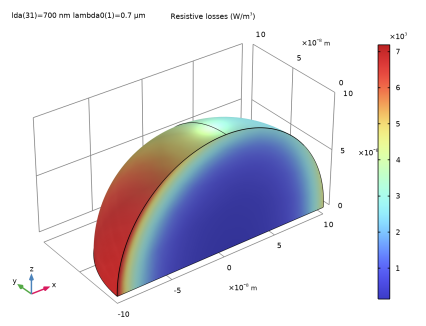
Select the Resolve wave in lossy media checkbox, to resolve the field down to the skin depth in the gold sphere.
|
|
1
|
|
2
|
|
3
|
Click
|
|
1
|
|
2
|
|
3
|
|
4
|
|
1
|
In the Electric Field (ewfd) toolbar, click
 |
|
1
|
|
2
|
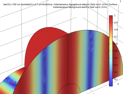
In the Electric Field, Background (ewfd) toolbar, click
 |
|
1
|
|
2
|
|
3
|
|
1
|
|
2
|
|
3
|
|
4
|
|
5
|
|
7
|
|
1
|
|
2
|
|
3
|
|
4
|
|
5
|
Select the Show legends checkbox.
|
|
1
|
|
2
|
|
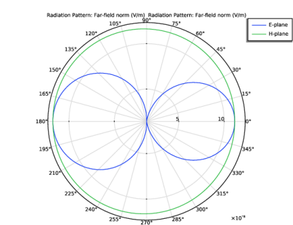
4
|
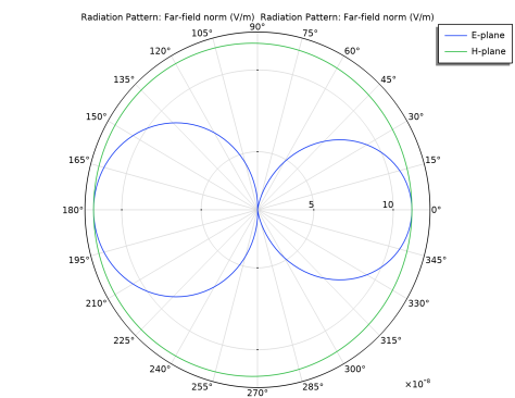
In the 2D Far Field (ewfd) toolbar, click
 |
|
1
|
|
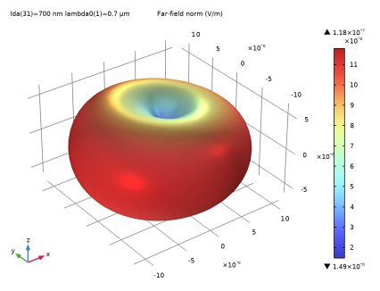
2
|
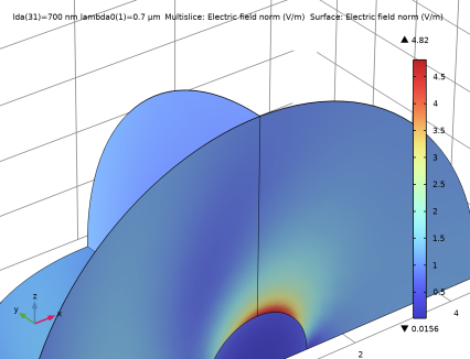
In the 3D Far Field (ewfd) toolbar, click
 |
|
1
|
|
2
|
|
1
|
|
2
|
|
3
|
|
4
|
|
5
|
|
6
|
|
1
|
|
2
|
|
3
|
|
4
|
|
6
|
Select the Apply to dataset edges checkbox.
|
|
1
|
|
2
|
In the Settings window for Volume, click Replace Expression in the upper-right corner of the Expression section. From the menu, choose Component 1 (comp1) > Electromagnetic Waves, Frequency Domain > Heating and losses > ewfd.Qrh - Resistive losses - W/m³.
|
|
3
|
|
4
|
Click the
 |
|
1
|
|
2
|
|
1
|
|
2
|
|
3
|
Click
|
|
4
|
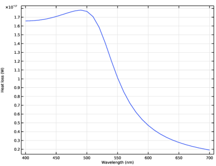
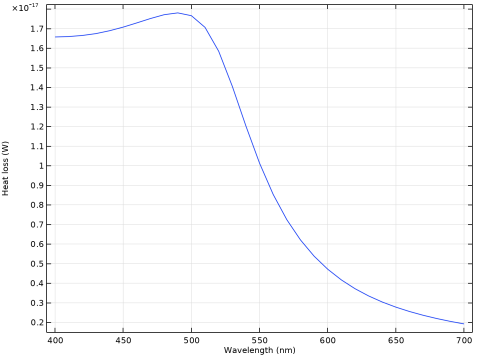
Click Replace Expression in the upper-right corner of the y-Axis Data section. From the menu, choose Component 1 (comp1) > Electromagnetic Waves, Frequency Domain > Heating and losses > ewfd.Ploss - Power loss - W. This variable represents the total integrated loss in the physics.
|
|
5
|
|
1
|
|
2
|
|
3
|
|
4
|
|
5
|
|
1
|
|
2
|
|
3
|
Locate the Plot Settings section.
|
|
4
|
|
1
|
|
2
|
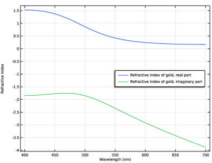
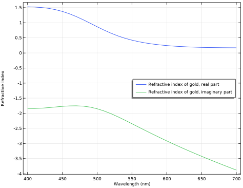
In the Settings window for Global, click Replace Expression in the upper-right corner of the y-Axis Data section. From the menu, choose Component 1 (comp1) > Definitions > Variables > n_gold - Refractive index of gold - 1.
|
|
3
|
Locate the y-Axis Data section. In the table, enter the following settings:
|
|
4
|
|
5
|
|
7
|
|
1
|
|
2
|
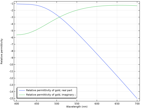
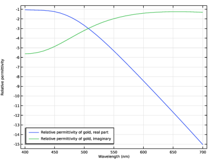
In the Settings window for 1D Plot Group, type Relative Permittivity of Gold in the Label text field.
|
|
1
|
|
2
|
In the Settings window for Global, click Replace Expression in the upper-right corner of the y-Axis Data section. From the menu, choose Component 1 (comp1) > Definitions > Variables > epsilonr_gold - Relative permittivity of gold - 1.
|
|
3
|
Locate the y-Axis Data section. In the table, enter the following settings:
|
|
4
|
Locate the Legends section. In the table, enter the following settings:
|
|
1
|
|
2
|
|
3
|
|
4
|
|
5
|
In the Relative Permittivity of Gold toolbar, click
 |
|
1
|
|
2
|
|
3
|
|
1
|
|
2
|
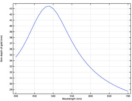
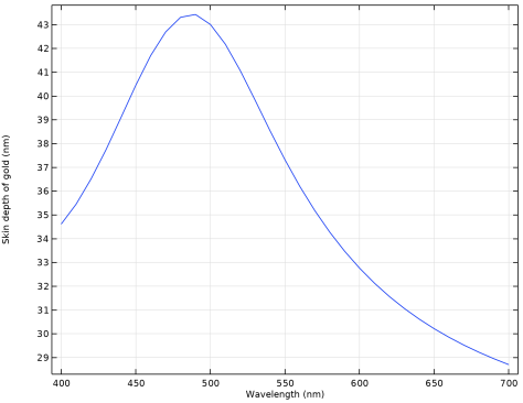
In the Settings window for Global, click Replace Expression in the upper-right corner of the y-Axis Data section. From the menu, choose Component 1 (comp1) > Definitions > Variables > deltaS_gold - Skin depth of gold - m.
|
|
3
|
Locate the y-Axis Data section. In the table, enter the following settings:
|
|
4
|