PDF

Defining a Mapped Dielectric Distribution of a Material
Introduction
This example demonstrates how to set up a spatially varying dielectric distribution, such as might be engineered with a metamaterial. Here, a convex lens shape is defined via a known deformation of a rectangular domain. The dielectric distribution is defined on the undeformed, original rectangular domain and is mapped onto the deformed shape of the lens. Although the lens shape defined here is convex, the dielectric distribution causes the incident beam to diverge.
Figure 1: A convex metamaterial lens. Both the shape and the dielectric distribution are defined on a rectangular domain, and mapped into the deformed state.
Model Definition
Consider a 2D model geometry as shown in Figure 2. A square air domain, bounded by a perfectly matched layer (PML) on all sides, encloses a rectangular region in which the metamaterial lens is defined.
Figure 2: The modeling domain consists of the metamaterial lens in an air domain, and a surrounding PML. A Gaussian beam is incident from the left.
Model a Gaussian beam entering the domain from the left side, via a surface current excitation at an interior boundary. The surface current, Js0, can also be thought of as a displacement current excitation. The waist of the beam is at the boundary, so the excitation at this boundary can be specified as
where w0 is the waist size. The excitation is at the boundary between a domain of free space and the PML, and excites a wave propagating in both directions — into the PML and into the modeling domain. The wave propagating into the PML is completely absorbed, and the wave propagating into the domain is diffracted by the lens.
Both the shape and the dielectric distribution of the metamaterial lens are defined with respect to the original Cartesian coordinate system, as shown in Figure 1. The true shape of the lens is described by the relationship
where Xg, Yg are the Cartesian coordinates of the undeformed frame.
The dielectric distribution is defined on the original Cartesian domain as:
The above expression introduces a variation in the dielectric in the y-coordinate of the undeformed lens. On the deformed lens, the dielectric varies in both directions.
The Deformed Geometry uses the above expressions to define the shape of the lens and maps the Cartesian coordinates of the undeformed frame onto the deformed frame. The dielectric distribution is defined with respect to the undeformed frame, and then mapped onto the deformed shape using the above expressions.
Results and Discussion
The model is solved for the out-of-plane electric field. Figure 3 plots the electric field norm, showing a Gaussian beam with minimal divergence incident upon the lens from the left. The beam is diffracted by the convex lens and spreads out.
Figure 4 displays the dielectric distribution, and shows variation in both directions defined via the mapping described above.
Figure 3: The norm of the electric field shows the Gaussian beam diffracted by the metamaterial lens.
Figure 4: Contour plot of the dielectric distribution.
Application Library path: Wave_Optics_Module/Gratings_and_Metamaterials/mapped_dielectric_distribution
Modeling Instructions
From the File menu, choose New.
New
In the New window, click  Model Wizard.
Model Wizard
1
In the Model Wizard window, click  2D.
2
In the Select Physics tree, select Optics > Wave Optics > Electromagnetic Waves, Frequency Domain (ewfd).
3
Click Add.
4
Click  Study.
5
In the Select Study tree, select Empty Study.
6
Global Definitions
Parameters 1
1
In the Model Builder window, under Global Definitions click Parameters 1.
2
In the Settings window for Parameters, locate the Parameters section.
3
Here, c_const is a predefined COMSOL constant for the speed of light in vacuum.
Geometry 1
First, create a square for the entire model domain. Add a layer on each side of the square.
Square 1 (sq1)
1
In the Geometry toolbar, click  Square.
2
In the Settings window for Square, locate the Size section.
3
In the Side length text field, type 3.
4
Locate the Position section. From the Base list, choose Center.
5
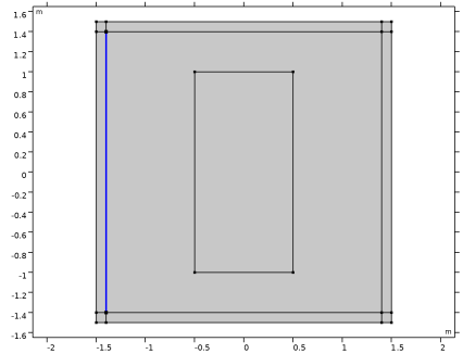
Click to expand the Layers section. In the table, enter the following settings:
6
Select the Layers to the left checkbox.
7
Select the Layers to the right checkbox.
8
Select the Layers on top checkbox.
9
Click  Build Selected.
Rectangle 1 (r1)
Add a rectangle for the lens.
1
In the Geometry toolbar, click  Rectangle.
2
In the Settings window for Rectangle, locate the Size and Shape section.
3
In the Height text field, type 2.
4
Locate the Position section. From the Base list, choose Center.
5
Click  Build All Objects.
Definitions
Lens
Add a selection for the lens domain which will be recalled frequently while setting up the model properties.
1
In the Definitions toolbar, click  Explicit.
2
In the Settings window for Explicit, type Lens in the Label text field.
3
Variables 1
Next, add a set of variables for the shape and the dielectric distribution of the lens.
1
In the Definitions toolbar, click  Local Variables.
2
In the Settings window for Variables, locate the Geometric Entity Selection section.
3
From the Geometric entity level list, choose Domain.
4
From the Selection list, choose Lens.
5
Locate the Variables section. In the table, enter the following settings:
Here, Xg and Yg are predefined Deformed Geometry physics variables representing the Cartesian coordinates of the undeformed frame.
Perfectly Matched Layer 1 (pml1)
Add a perfectly matched layer (PML).
1
In the Definitions toolbar, click  Perfectly Matched Layer.
2
Set up Deformed geometry. You need to specify Deforming Domain, Prescribed Deformation.
Component 1 (comp1)
Deforming Domain 1
1
In the Physics toolbar, click  Deformed Geometry and choose Free Deformation.
2
3
In the Settings window for Deforming Domain, locate the Smoothing section.
4
From the Mesh smoothing type list, choose Laplace.
Prescribed Deformation 1
1
In the Deformed Geometry toolbar, click  Prescribed Deformation.
2
3
In the Settings window for Prescribed Deformation, locate the Prescribed Deformation section.
4
Specify the dx vector as
Electromagnetic Waves, Frequency Domain (ewfd)
In Electromagnetic Waves, Frequency Domain, the dielectric distribution is configured via the user-defined variable erp and the Gaussian beam is modeled as entering the domain from the left side, via a surface current excitation.
1
In the Model Builder window, under Component 1 (comp1) click Electromagnetic Waves, Frequency Domain (ewfd).
2
In the Settings window for Electromagnetic Waves, Frequency Domain, locate the Components section.
3
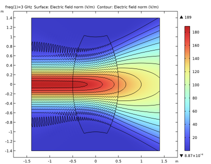
From the Electric field components solved for list, choose Out-of-plane vector to only perform the calculation for the out-of-plane component. The in-plane components are both zero.
Wave Equation, Electric 2
1
In the Physics toolbar, click  Domains and choose Wave Equation, Electric.
2
In the Settings window for Wave Equation, Electric, locate the Domain Selection section.
3
From the Selection list, choose Lens.
4
Locate the Electric Displacement Field section. From the Electric displacement field model list, choose Relative permittivity.
5
From the εr list, choose User defined. In the associated text field, type erp.
6
Locate the Magnetic Field section. From the μr list, choose User defined. Leave the default value 1.
7
Locate the Conduction Current section. From the σ list, choose User defined. Leave the default value 0.
Surface Current Density 1
1
In the Physics toolbar, click  Boundaries and choose Surface Current Density.
2
3
In the Settings window for Surface Current Density, locate the Surface Current Density section.
4
Specify the Js0 vector as
Materials
Set all domain with vacuum. The lens domain material properties are explicitly configured by Wave Equation, Electric 2 in Electromagnetic Waves, Frequency Domain.
Add Material
1
In the Materials toolbar, click  Add Material to open the Add Material window.
2
Go to the Add Material window.
3
In the tree, select Built-in > Air.
4
Click the Add to Component button in the window toolbar.
5
In the Materials toolbar, click  Add Material to close the Add Material window.
Mesh 1
Free Triangular 1
1
In the Mesh toolbar, click  Free Triangular.
2
In the Settings window for Free Triangular, locate the Domain Selection section.
3
From the Geometric entity level list, choose Domain.
4
Size
1
In the Model Builder window, click Size.
2
In the Settings window for Size, locate the Element Size section.
3
Click the Custom button.
4
Locate the Element Size Parameters section. In the Maximum element size text field, type lda0/10.
5
In the Minimum element size text field, type 0.0012.
Mapped 1
In the Mesh toolbar, click  Mapped.
Distribution 1
1
Right-click Mapped 1 and choose Distribution.
2
3
In the Settings window for Distribution, locate the Distribution section.
4
In the Number of elements text field, type 10.
5
Click  Build All. You may zoom in a few times to check the quality of the mesh.
The model is analyzed with two study steps. First, make sure that Stationary study step is solved only for Deformed Geometry.
Study 1
Step 1: Stationary
In the Study toolbar, click  Stationary.
Step 2: Frequency Domain
Add a Frequency Domain study step and set as solve only for Electromagnetic Waves, Frequency Domain.
1
In the Study toolbar, click  Frequency Domain.
2
In the Settings window for Frequency Domain, locate the Study Settings section.
3
In the Frequencies text field, type f0.
4
Locate the Physics and Variables Selection section. In the Solve for column of the table, under Component 1 (comp1), clear the checkbox for Deformed Geometry.
5
In the Study toolbar, click  Compute.
Results
Electric Field (ewfd)
The default plot shows the magnitude of electric fields. Add a contour plot for the magnitude.
Contour 1
1
Right-click Electric Field (ewfd) and choose Contour.
2
In the Settings window for Contour, locate the Levels section.
3
In the Total levels text field, type 14.
4
Locate the Coloring and Style section. From the Coloring list, choose Uniform.
5
From the Color list, choose Black.
6
Clear the Color legend checkbox.
7
In the Electric Field (ewfd) toolbar, click  Plot. See Figure 3 to compare the reproduced plot.
2D Plot Group 3
Add a filled contour plot describing the dielectric distribution over the lens.
1
In the Results toolbar, click  2D Plot Group.
2
In the Settings window for 2D Plot Group, click to expand the Selection section.
3
From the Geometric entity level list, choose Domain.
4
5
Select the Apply to dataset edges checkbox.
Contour 1
1
Right-click 2D Plot Group 3 and choose Contour.
2
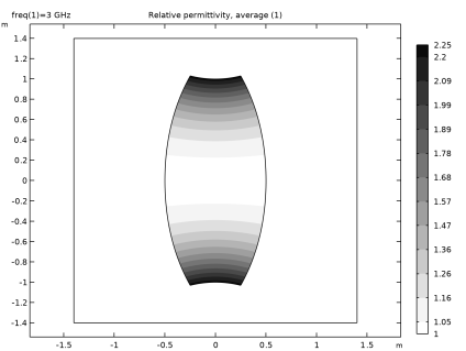
In the Settings window for Contour, click Replace Expression in the upper-right corner of the Expression section. From the menu, choose Component 1 (comp1) > Electromagnetic Waves, Frequency Domain > Material properties > ewfd.epsrAv - Relative permittivity, average - 1.
3
Locate the Levels section. In the Total levels text field, type 12.
4
Locate the Coloring and Style section. From the Contour type list, choose Filled.
5
From the Color table list, choose GrayScale.
6
From the Color table transformation list, choose Reverse.
7
In the 2D Plot Group 3 toolbar, click  Plot.
8
Click the  Zoom Extents button in the Graphics toolbar. The plot for the dielectric distribution is shown in Figure 4.