PDF

Reflection of a Circularly Polarized Plane Wave
Introduction
A circularly polarized plane wave is reflected and transmitted at a boundary between air and a dielectric material. This model demonstrates how to solve this problem using three different approaches:
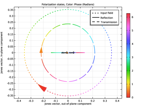
with a Periodic structure feature, specifying the circular polarization for the incident wave
This example demonstrates that the simplest way to correctly model this problem is to use the Periodic Structure feature.
Starting from the theoretical framework described in the Fresnel Equations model, comparisons show excellent agreement between the computed results and analytical expressions for the polarization state of the reflected and transmitted waves.
A plane wave propagating in an isotropic homogeneous material can have a polarization state that is the superposition of two orthogonal polarization base states. The simplest polarization base states are linear polarization states. Here, the electric field vector oscillates in a plane that is constant along the propagation direction.
As in this case, the incident wave is reflected and refracted at an interface between two different materials, it is common to define the two orthogonal polarization states as the out-of-plane s- or TE-polarization and the in-plane p- or TM-polarization. The s-polarization is directed in the out-of-plane direction with respect to the plane of incidence, defined by the propagation direction and the normal to the interface plane. The p-polarization is pointing in a direction parallel to the plane of incidence.
If you add s- and p-polarizations with equal amplitudes and with a π/2 phase shift, you get circular polarization. If you monitor the electric field amplitude vector at a point in space as a function of time, the amplitude vector tip will rotate along a circle. Thereby the name, circular polarization. For right-handed circular polarization (RHCP), if you align the thumb of the right hand in the propagation direction, away from the source, the other fingers align in the direction the amplitude vector rotates as a function of time. Similarly, for left-handed circular polarization (LHCP), you align the left hand thumb in the propagation direction and the amplitude vector rotates as a function of time in the direction of the other fingers on the left hand.
Model Definition
An incident plane wave with pure RHCP propagates through air (n_air = 1). At the interface between air and the dielectric (n_slab = 1.5), the wave is split into a reflected wave and a transmitted (refracted) wave (see Figure 1).
Figure 1: The incident and reflected waves propagate in air, whereas the transmitted wave propagates in an infinitely thick dielectric medium. The incident wave has pure right-handed circular polarization (RHCP), whereas the reflected wave has a mix of left-handed circular polarization (LHCP) and some RHCP. The transmitted wave has mostly RHCP, but also some LHCP. The rings with crosses or dots represent s-polarization directions into or out from the page and the short in-plane arrows represent p-polarization directions for the respective waves. The rings with a small arrow represent the circular polarization state, watching the polarization vector rotate as a function of time when looking in the propagation direction of the respective waves.
Circular polarization consists of equal amplitudes of s- and p-polarization. However, for non-normal angles of incidence, the reflection and transmission coefficients for s- and p-polarizations are different. This is described in more detail in the Fresnel Equations model. The effect is that the reflected and transmitted waves don’t contain a single circular polarization state, but a mix of RCHP and LHCP.
The transmitted wave consists of mostly RHCP, but also some LHCP.
The amplitude vector for the reflected wave rotates in the same direction as the amplitude vector of the incident wave. However, since the propagation directions are different, the reflected wave consists mostly of LCHP, but with some RHCP. The amount of LHCP and RHCP depends on the angle of incidence.
At the Brewster angle, the reflection coefficient for p-polarization is zero. Thus, at that angle, the reflected wave is purely s-polarized. Another way of describing the polarization at the Brewster angle is to say that the reflected wave consists of equal amounts of RHCP and LHCP and that the superposition of those two circular polarization states generates a pure s-polarization.
Mathematically, the incident wave can be described by the summation of equal amplitudes of s- and p-polarization,
(1),
where E0 is the amplitude; us, up, and uR are the polarization directions for s-, p-, and right-handed circular polarization, respectively; kin is the wave vector for the incident wave; and r is the position vector. Note that the RHCP direction is formed by adding the s- and p-polarization directions with the π/2 phase difference (the factor j).
The polarization direction for LHCP is given by
(2).
Using the Fresnel reflection coefficients, defined and discussed in the Fresnel Equations model, the reflected wave is written as
(3).
Identifying the coefficients belonging to the respective s- and p-polarization vectors, the following two relations can be derived for the reflection coefficients
(4)
and
(5).
From these equations, the reflection coefficients for the circular polarizations can be deduced as
(6)
and
(7).
Since the dielectric has a larger refractive index than air, the reflection coefficient for s-polarization, rs, is negative, whereas the reflection coefficient for p-polarization is positive for small angles of incidence. Thereby, for small angles of incidence, the reflection coefficient for LHCP will be larger than the reflection coefficient for RHCP. However, for angles of incidence larger than the Brewster angle, also the reflection coefficient for p-polarization, rp, is negative. Then the reflection coefficient for RHCP will be larger than the reflection coefficient for LHCP.
In COMSOL, the mode fields are specified for the outgoing waves — both for the excitation port and the ports without excitation. Because of the different propagation directions for the incoming and the outgoing waves, the same mode fields represents different polarization states for the incoming and the outgoing waves. Thus, to specify an incoming waves with RHCP, you should specify a mode field for the outgoing wave with LHCP. Furthermore, as circular polarization can be decomposed into a superposition of s- and p-polarizations and the reflection and transmission coefficients are different for the two polarizations for non-normal incidence, at each port boundary both a Port node and an Orthogonal Polarization node must be added to handle the fact that the reflection/transmission coefficients are different for the two polarizations.
This model describes three different ways to solve this problem. First, Port nodes with user-defined electric mode field amplitudes are used. Now, it is important to define the components of the LHCP for the excitation port and RHCP for the listener port.
S-polarization means that the electric field vector is orthogonal to the plane of incidence, which is spanned by the normal to the interface between the two media and the propagation direction. Thus, we can define the s-polarization vector as
(8)
where k is the wave vector for any of the incident, reflected, or transmitted waves, kT is the component of the wave vector that is tangential to the port boundary (pointing in the x-direction and the same for all the waves), n is the port normal (pointing out from the physics) and y is the unit vector in the y-direction. The minus sign is used for the excitation port, as there n = z, whereas the plus sign is used on the opposite port boundary, as there n = z.
The p-polarization vector should be orthogonal to both the s-polarization vector and the propagation direction. Thus, it can be defined as
(9)
So, for Port 1, the excitation port, a mode field amplitude representing LHCP is defined by
(10).
Similarly, for Port 2, the listener port, a mode field amplitude representing RHCP is defined as
(11).
The second approach to model this problem is to specify what kind of circular polarization that will be used by the two ports. The advantage is of course that the electric field amplitude components are automatically defined. However, also in this case it is important to realize that it is the polarization state for the outgoing wave that is specified. Thus, specify LHCP and RHCP for ports 1 and 2, respectively.
The third and final approach to model this problem is to use the Periodic Structure node. This is a domain feature that automatically adds all required subnodes, like ports and periodic boundary conditions. Here, it is the polarization of the incident — or dominant — polarization that is specified. Based on this specification, the polarization states for the port subnodes are automatically assigned.
It is highly recommended to use the Periodic Structure node when defining periodic problems, as it automatically defines the proper settings for the ports and the periodic conditions. The first two, more manual, approaches, however, are good for getting a more detailed understanding of how the ports are configured to solve the problem correctly.
Results and Discussion
Figure 2 shows the Cartesian components of the electric field distributions, as calculated with the three different modeling approaches. It is clear that all three approaches result in very similar solutions.
Figure 2: Plot of the Cartesian components of the electric fields for the three different modeling approaches. The different plots along the x-direction show the electric field distributions for the different Cartesian components, whereas the plots along the y-direction show the results for the different modeling approaches.
Figure 3 shows the reflectance and transmittance for the different circular polarization states. For small angles of incidence, the reflectance for LHCP is larger than the reflectance for RHCP. At the Brewster angle, the reflectances for the two circular polarization states are equally large, forming a pure s-polarization for the reflected wave. For angles larger than the Brewster angle, the reflectance for RHCP is larger than the reflectance for LHCP.
The markers represent the analytical solutions, based on Equation 6 and Equation 7. As expected, the analytical values and the results from the full-wave solutions agree very well.
Figure 3: Reflectance and transmittance curves for the different circular polarization states.
Figure 4 shows the polarization plot at the Brewster angle. It is clear that the reflected wave has a pure out-of-plane (s) polarization.
To understand what kind of circular polarization that is shown in the plot, point the right hand thumb into the page (screen). As the rest of the right-hand fingers align with the arrows in the plots for the input and transmitted waves, the input wave is purely RHCP and the transmitted wave is mostly RHCP. For an LHCP wave, the left hand fingers align with the arrow, when the thumb points into the page.
Figure 4: Plot of the polarization states for the input (dotted line), reflected (solid line), and transmitted (dashed line) waves at the Brewster angle.
Application Library path: Wave_Optics_Module/Verification_Examples/circular_polarization
Modeling Instructions
From the File menu, choose New.
New
In the New window, click  Model Wizard.
Model Wizard
1
In the Model Wizard window, click  3D.
2
In the Select Physics tree, select Optics > Wave Optics > Electromagnetic Waves, Frequency Domain (ewfd).
3
Click Add.
4
Click  Study.
5
In the Select Study tree, select Preset Studies for Selected Physics Interfaces > Wavelength Domain.
6
Global Definitions
Parameters 1
1
In the Model Builder window, under Global Definitions click Parameters 1.
2
In the Settings window for Parameters, locate the Parameters section.
3
Click  Load from File.
4
Geometry 1
Block 1 (blk1)
1
In the Geometry toolbar, click  Block.
2
In the Settings window for Block, locate the Size and Shape section.
3
In the Width text field, type a0.
4
In the Depth text field, type a0.
5
In the Height text field, type b0.
6
Click to expand the Layers section. In the table, enter the following settings:
7
Click  Build All Objects.
This creates a rectangular geometry, consisting of two layers. The top domain consists of air and the bottom domain consists of glass.
Materials
Air
1
In the Model Builder window, under Component 1 (comp1) right-click Materials and choose Blank Material.
2
In the Settings window for Material, type Air in the Label text field.
3
Locate the Material Contents section. In the table, enter the following settings:
Glass
1
Right-click Materials and choose Blank Material.
2
In the Settings window for Material, type Glass in the Label text field.
3
4
Locate the Material Contents section. In the table, enter the following settings:
Electromagnetic Waves, Frequency Domain (ewfd)
Now, define the first physics interface. Here, periodic Port features will be used, with user-defined settings for the port mode field amplitudes.
Port 1
1
In the Physics toolbar, click  Boundaries and choose Port.
2
3
In the Settings window for Port, locate the Boundary Selection section.
4
Click  Create Selection, as this selection will be reused later.
5
In the Create Selection dialog, type Port 1 in the Selection name text field.
6
7
In the Settings window for Port, locate the Port Properties section.
8
From the Type of port list, choose Periodic.
9
Locate the Port Mode Settings section. Specify the E0 vector as
These settings create a mode field amplitude that is orthogonal to the wave vector for the outgoing wave. The s-polarization (TE) is defined by the y component and the x and z components define the p-polarization (TM). Because the amplitudes for the s- and p-polarizations are of equal magnitude and there is a π/2 phase shift between the two linear polarizations, these settings will define a left-handed circular polarization for the outgoing wave. That means the incident wave will have right-handed circular polarization.
10
In the α1 text field, type alpha.
Port 2
1
In the Physics toolbar, click  Boundaries and choose Port.
2
3
In the Settings window for Port, locate the Boundary Selection section.
4
Click  Create Selection.
5
In the Create Selection dialog, type Port 2 in the Selection name text field.
6
7
In the Settings window for Port, locate the Port Properties section.
8
From the Type of port list, choose Periodic.
9
Locate the Port Mode Settings section. Specify the E0 vector as
These settings define a right-handed circular polarization for the outgoing wave at the second port.
Port 1
Now, define Orthogonal Polarization ports, as subnodes to the two periodic Port nodes. These Orthogonal Polarization ports will absorb the radiation that does not match the mode fields of the periodic Port nodes.
In the Model Builder window, click Port 1.
Orthogonal Polarization 1
In the Physics toolbar, click  Attributes and choose Orthogonal Polarization.
Port 2
In the Model Builder window, under Component 1 (comp1) > Electromagnetic Waves, Frequency Domain (ewfd) click Port 2.
Orthogonal Polarization 1
In the Physics toolbar, click  Attributes and choose Orthogonal Polarization.
Periodic Condition 1
1
In the Physics toolbar, click  Boundaries and choose Periodic Condition.
2
3
In the Settings window for Periodic Condition, locate the Boundary Selection section.
4
Click  Create Selection.
5
In the Create Selection dialog, type Periodic Condition 1 in the Selection name text field.
6
7
In the Settings window for Periodic Condition, locate the Periodicity Settings section.
8
From the Type of periodicity list, choose Floquet periodicity.
9
From the k-vector for Floquet periodicity list, choose From periodic port.
Periodic Condition 2
1
Right-click Periodic Condition 1 and choose Duplicate.
2
In the Settings window for Periodic Condition, locate the Boundary Selection section.
3
Click  Clear Selection.
4
5
Click  Create Selection.
6
In the Create Selection dialog, type Periodic Condition 2 in the Selection name text field.
7
Study 1
Step 1: Wavelength Domain
1
In the Model Builder window, under Study 1 click Step 1: Wavelength Domain.
2
In the Settings window for Wavelength Domain, locate the Study Settings section.
3
In the Wavelengths text field, type lda0.
4
Click to expand the Study Extensions section. Select the Auxiliary sweep checkbox.
5
6
Here, the Brewster angle parameter alpha_Brewster was included in the angle sweep.
7
In the Study toolbar, click  Compute.
Results
Electric Field (ewfd)
Next, modify the default plot group Electric Field (ewfd) to plot the electric field components, instead of the electric field norm.
1
In the Settings window for 3D Plot Group, click to expand the Plot Array section.
2
From the Array type list, choose Linear.
Multislice 1
1
In the Model Builder window, expand the Electric Field (ewfd) node, then click Multislice 1.
2
In the Settings window for Multislice, locate the Expression section.
3
In the Expression text field, type ewfd.Ex.
4
Locate the Coloring and Style section. From the Color table list, choose WaveLight.
5
From the Scale list, choose Linear symmetric.
Multislice 2
1
Right-click Results > Electric Field (ewfd) > Multislice 1 and choose Duplicate.
2
In the Settings window for Multislice, locate the Expression section.
3
In the Expression text field, type ewfd.Ey.
4
Click to expand the Inherit Style section. From the Plot list, choose Multislice 1.
Multislice 3
1
Right-click Multislice 2 and choose Duplicate.
2
In the Settings window for Multislice, locate the Expression section.
3
In the Expression text field, type ewfd.Ez.
Electric Field (ewfd)
1
In the Model Builder window, click Electric Field (ewfd).
2
In the Settings window for 3D Plot Group, locate the Data section.
3
From the Parameter value (alpha (deg)) list, choose 45.
4
Click to expand the Title section. From the Title type list, choose Manual.
5
In the Title text area, type Multislice: Electric field, Cartesian components (V/m).
6
In the Parameter indicator text field, type lambda0=1 µm, alpha=45 deg.
7
Locate the Plot Settings section. Clear the Plot dataset edges checkbox.
8
Click the  Show Grid button in the Graphics toolbar.
9
Click the  Zoom Extents button in the Graphics toolbar.
10
In the Electric Field (ewfd) toolbar, click  Plot.
This plot shows that the s (TE) polarization (y component) is out-of-phase with respect to the p (TM) polarization (x and z components).
Reflectance and Transmittance (ewfd)
1
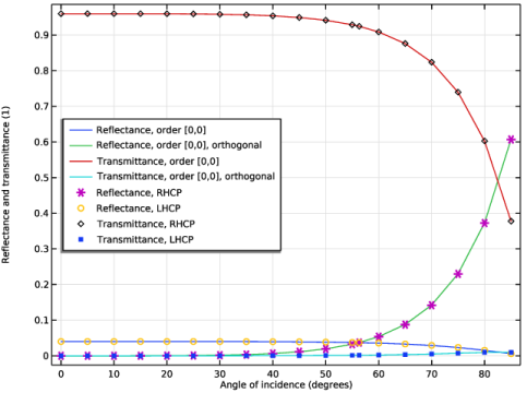
In the Model Builder window, under Results click Reflectance, Transmittance, and Absorptance (ewfd).
2
In the Settings window for 1D Plot Group, type Reflectance and Transmittance (ewfd) in the Label text field.
Global 1
1
In the Model Builder window, expand the Reflectance and Transmittance (ewfd) node, then click Global 1.
2
In the Settings window for Global, locate the y-Axis Data section.
3
Ctrl-click to select table rows 3 and 6–8. That is, select the expressions ewfd.Rtotal, ewfd.Ttotal, ewfd.RTtotal, and ewfd.Atotal.
4
Click  Delete.
Global 2
1
In the Model Builder window, right-click Reflectance and Transmittance (ewfd) and choose Global.
2
In the Settings window for Global, locate the y-Axis Data section.
3
4
Click to expand the Coloring and Style section. Find the Line style subsection. From the Line list, choose None.
5
Find the Line markers subsection. From the Marker list, choose Cycle.
6
Click to expand the Legends section. Find the Include subsection. Clear the Solution checkbox.
Reflectance and Transmittance (ewfd)
1
In the Model Builder window, click Reflectance and Transmittance (ewfd).
2
In the Settings window for 1D Plot Group, locate the Plot Settings section.
3
Select the x-axis label checkbox. In the associated text field, type Angle of incidence (degrees).
4
In the y-axis label text field, type Reflectance and transmittance (1).
5
Locate the Legend section. From the Position list, choose Middle left.
6
In the Reflectance and Transmittance (ewfd) toolbar, click  Plot.
It is clear that the results from the full-field model and the analytical results agree very well.
Polarization Plot (ewfd)
1
In the Model Builder window, click Polarization Plot (ewfd).
For normal incidence, both the reflected and the transmitted waves have perfectly circular polarization. However, as the arrows point in opposite directions, it is clear that the reflected and transmitted waves have opposite circular polarizations, LHCP and RHCP, respectively. As expected, the input field is RHCP. The size of the circles also indicates that most of the incident intensity is transmitted.
2
In the Settings window for 1D Plot Group, locate the Data section.
3
In the Parameter values (alpha (deg)) list box, select 56.31, which corresponds to the Brewster angle.
4
In the Polarization Plot (ewfd) toolbar, click  Plot.
At the Brewster angle, the in-plane polarization component for the reflected wave is zero. Thus, the plot shows that the reflected wave has linear polarization in the out-of-plane direction.
Component 1 (comp1)
Now, add another physics interface. This time, the circular polarization will be specified by directly picking the appropriate polarization state from the Port settings.
Add Physics
1
In the Home toolbar, click  Add Physics to open the Add Physics window.
2
Go to the Add Physics window.
3
In the tree, select Optics > Wave Optics > Electromagnetic Waves, Frequency Domain (ewfd).
4
Find the Physics interfaces in study subsection. In the table, clear the Solve checkbox for Study 1.
5
Click the Add to Component 1 button in the window toolbar.
6
In the Home toolbar, click  Add Physics to close the Add Physics window.
Electromagnetic Waves, Frequency Domain 2 (ewfd2)
Port 1
1
In the Physics toolbar, click  Boundaries and choose Port.
2
In the Settings window for Port, locate the Boundary Selection section.
3
From the Selection list, choose Port 1.
4
Locate the Port Properties section. From the Type of port list, choose Periodic.
5
Locate the Port Mode Settings section. From the Polarization list, choose Circular polarization.
Notice that the default Circular polarization for the excited port is Left-handed. Since this specifies the polarization of the outgoing/reflected waves, the incoming wave will be a right-handed circularly polarized plane wave.
6
In the α1 text field, type alpha.
Port 2
1
In the Physics toolbar, click  Boundaries and choose Port.
2
In the Settings window for Port, locate the Boundary Selection section.
3
From the Selection list, choose Port 2.
4
Locate the Port Properties section. From the Type of port list, choose Periodic.
5
Locate the Port Mode Settings section. From the Polarization list, choose Circular polarization.
For the Port node on the transmission side, the default Circular polarization is Right-handed, which is consistent with right-handed circular polarization for the incoming wave at the excitation port.
Port 1
In the Model Builder window, click Port 1.
Orthogonal Polarization 1
In the Physics toolbar, click  Attributes and choose Orthogonal Polarization.
Port 2
In the Model Builder window, under Component 1 (comp1) > Electromagnetic Waves, Frequency Domain 2 (ewfd2) click Port 2.
Orthogonal Polarization 1
In the Physics toolbar, click  Attributes and choose Orthogonal Polarization.
Periodic Condition 1
1
In the Physics toolbar, click  Boundaries and choose Periodic Condition.
2
In the Settings window for Periodic Condition, locate the Boundary Selection section.
3
From the Selection list, choose Periodic Condition 1.
4
Locate the Periodicity Settings section. From the Type of periodicity list, choose Floquet periodicity.
5
From the k-vector for Floquet periodicity list, choose From periodic port.
Periodic Condition 2
1
Right-click Periodic Condition 1 and choose Duplicate.
2
In the Settings window for Periodic Condition, locate the Boundary Selection section.
3
From the Selection list, choose Periodic Condition 2.
Add Study
1
In the Home toolbar, click  Add Study to open the Add Study window.
2
Go to the Add Study window.
3
Find the Studies subsection. In the Select Study tree, select Preset Studies for Selected Physics Interfaces > Wavelength Domain.
4
Find the Physics interfaces in study subsection. In the table, clear the Solve checkbox for Electromagnetic Waves, Frequency Domain (ewfd).
5
Click the Add Study button in the window toolbar.
6
In the Home toolbar, click  Add Study to close the Add Study window.
Study 2
Step 1: Wavelength Domain
1
In the Settings window for Wavelength Domain, locate the Study Settings section.
2
In the Wavelengths text field, type lda0.
3
Locate the Study Extensions section. Select the Auxiliary sweep checkbox.
4
5
This is easiest done by copying the Parameter value list cell contents from the Study Extensions settings in Step 1: Wavelength Domain under Study 1 and then pasting the value into this table.
6
In the Study toolbar, click  Compute.
Results
Electric Field (ewfd, ewfd2)
1
In the Model Builder window, under Results click Electric Field (ewfd).
2
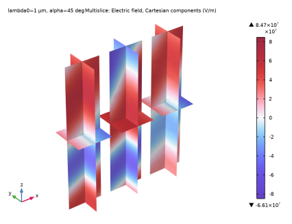
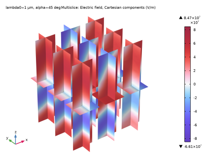
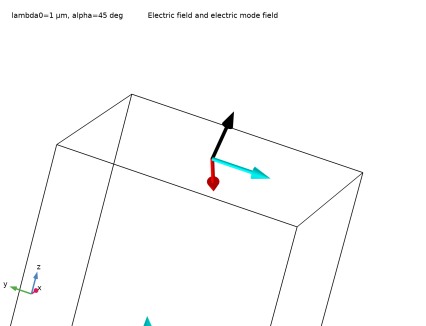
In the Settings window for 3D Plot Group, type Electric Field (ewfd, ewfd2) in the Label text field.
3
Locate the Plot Array section. From the Array type list, choose Square.
Multislice 4
1
In the Model Builder window, under Results > Electric Field (ewfd, ewfd2) right-click Multislice 3 and choose Duplicate.
2
In the Settings window for Multislice, locate the Data section.
3
From the Dataset list, choose Study 2/Solution 2 (sol2).
4
From the Parameter value (alpha (deg)) list, choose 45.
5
Locate the Expression section. In the Expression text field, type ewfd2.Ex.
Multislice 5
1
Right-click Multislice 4 and choose Duplicate.
2
In the Settings window for Multislice, locate the Expression section.
3
In the Expression text field, type ewfd2.Ey.
Multislice 6
1
Right-click Multislice 5 and choose Duplicate.
2
In the Settings window for Multislice, locate the Expression section.
3
In the Expression text field, type ewfd2.Ez.
4
Click the  Zoom Extents button in the Graphics toolbar.
5
In the Electric Field (ewfd, ewfd2) toolbar, click  Plot.
Notice that the field distributions are identical for the two different physics interfaces.
Electric Field (ewfd2)
In the Model Builder window, under Results right-click Electric Field (ewfd2) and choose Delete.
Reflectance and Transmittance (ewfd2)
In the Settings window for 1D Plot Group, type Reflectance and Transmittance (ewfd2) in the Label text field.
Global 1
1
In the Model Builder window, expand the Reflectance and Transmittance (ewfd2) node, then click Global 1.
2
In the Settings window for Global, locate the y-Axis Data section.
3
4
Click  Delete.
Global 2
In the Model Builder window, under Results > Reflectance and Transmittance (ewfd) right-click Global 2 and choose Copy.
Global 2
In the Model Builder window, right-click Reflectance and Transmittance (ewfd2) and choose Paste Global.
Reflectance and Transmittance (ewfd2)
1
In the Settings window for 1D Plot Group, locate the Plot Settings section.
2
Select the x-axis label checkbox. In the associated text field, type Angle of Incidence (degrees).
3
In the y-axis label text field, type Reflectance and transmittance (1).
4
Locate the Legend section. From the Position list, choose Middle left.
5
In the Reflectance and Transmittance (ewfd2) toolbar, click  Plot.
Again, the full-wave and the analytical results are in excellent agreement.
Component 1 (comp1)
Finally, add a third physics interface. This time, a Periodic Structure node will be used. This greatly simplifies the modeling process, as many of the previous modeling steps are now performed automatically.
Add Physics
1
In the Home toolbar, click  Add Physics to open the Add Physics window.
2
Go to the Add Physics window.
3
In the tree, select Recently Used > Electromagnetic Waves, Frequency Domain (ewfd).
4
Find the Physics interfaces in study subsection. In the table, clear the Solve checkboxes for Study 1 and Study 2.
5
Click the Add to Component 1 button in the window toolbar.
6
In the Home toolbar, click  Add Physics to close the Add Physics window.
Electromagnetic Waves, Frequency Domain 3 (ewfd3)
Periodic Structure 1
1
In the Physics toolbar, click  Domains and choose Periodic Structure.
2
In the Settings window for Periodic Structure, locate the Port Mode Settings section.
3
From the Polarization list, choose Circular polarization. As the default Circular polarization is Right-handed, this will define an incoming right-handed circularly polarized plane wave.
4
In the α1 text field, type alpha.
5
Expand the Periodic Structure 1 node, to see that the Periodic Structure node automatically creates Periodic Port and Floquet Periodic Condition subnodes.
6
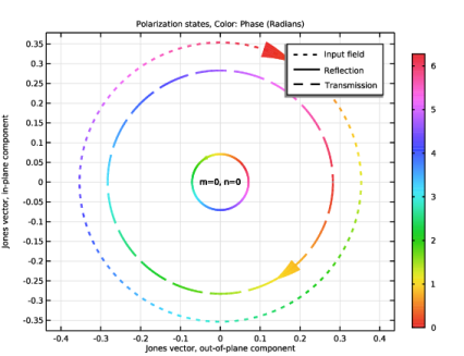
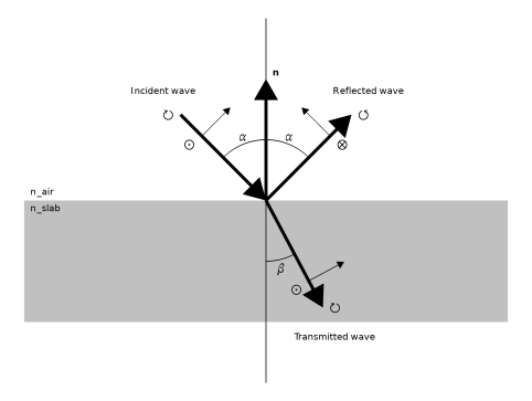
Select the Periodic Port 1 node. Since the Polarization setting on the Periodic Structure node represents the polarization state for the incident waves, the excited Periodic Port node automatically gets left-handed circular polarization as the setting on the Periodic Port node represents the state for the outgoing (reflected) wave. This is also consistent with how the polarization was specified for Port 1 for the Electromagnetic Waves, Frequency Domain 2 interface.
7
Select the Periodic Port 2 node, to see that Periodic Port automatically gets the same polarization as Port 2 in the Electromagnetic Waves, Frequency Domain 2 interface.
Add Study
1
In the Home toolbar, click  Add Study to open the Add Study window.
2
Go to the Add Study window.
3
Find the Studies subsection. In the Select Study tree, select Preset Studies for Selected Physics Interfaces > Wavelength Domain.
4
Find the Physics interfaces in study subsection. In the table, clear the Solve checkboxes for Electromagnetic Waves, Frequency Domain (ewfd) and Electromagnetic Waves, Frequency Domain 2 (ewfd2).
5
Click the Add Study button in the window toolbar.
6
In the Home toolbar, click  Add Study to close the Add Study window.
Study 3
Step 1: Wavelength Domain
1
In the Settings window for Wavelength Domain, locate the Study Settings section.
2
In the Wavelengths text field, type lda0.
3
Locate the Study Extensions section. Select the Auxiliary sweep checkbox.
4
5
Again, copy the angles for Parameter value list from any of the two previous Wavelength Domain study steps.
6
In the Study toolbar, click  Compute.
Results
Electric Field (ewfd, ewfd2, ewfd3)
1
In the Model Builder window, under Results click Electric Field (ewfd, ewfd2).
2
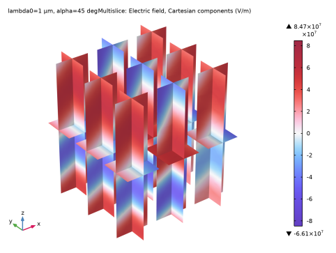
In the Settings window for 3D Plot Group, type Electric Field (ewfd, ewfd2, ewfd3) in the Label text field.
Multislice 7
1
In the Model Builder window, under Results > Electric Field (ewfd, ewfd2, ewfd3) right-click Multislice 4 and choose Duplicate.
2
In the Settings window for Multislice, locate the Data section.
3
From the Dataset list, choose Study 3/Solution 3 (sol3).
4
Locate the Expression section. In the Expression text field, type ewfd3.Ex.
Multislice 8
1
Right-click Multislice 7 and choose Duplicate.
2
In the Settings window for Multislice, locate the Expression section.
3
In the Expression text field, type ewfd3.Ey.
Multislice 9
1
Right-click Multislice 8 and choose Duplicate.
2
In the Settings window for Multislice, locate the Expression section.
3
In the Expression text field, type ewfd3.Ez.
4
In the Electric Field (ewfd, ewfd2, ewfd3) toolbar, click  Plot.
5
Click the  Zoom Extents button in the Graphics toolbar.
It is clear that the field distributions are almost the same for all three different modeling approaches.
Electric Field (ewfd3)
In the Model Builder window, under Results right-click Electric Field (ewfd3) and choose Delete.
Reflectance and Transmittance (ewfd3)
In the Settings window for 1D Plot Group, type Reflectance and Transmittance (ewfd3) in the Label text field.
Global 1
1
In the Model Builder window, expand the Reflectance and Transmittance (ewfd3) node, then click Global 1.
2
In the Settings window for Global, locate the y-Axis Data section.
3
4
Click  Delete.
Global 2
In the Model Builder window, under Results > Reflectance and Transmittance (ewfd) right-click Global 2 and choose Copy.
Global 2
In the Model Builder window, right-click Reflectance and Transmittance (ewfd3) and choose Paste Global.
Reflectance and Transmittance (ewfd3)
1
In the Settings window for 1D Plot Group, locate the Plot Settings section.
2
Select the x-axis label checkbox. In the associated text field, type Angle of incidence (degrees).
3
In the y-axis label text field, type Reflectance and transmittance (1).
4
Locate the Legend section. From the Position list, choose Middle left.
5
In the Reflectance and Transmittance (ewfd3) toolbar, click  Plot.
This plot confirms that all three ways of modeling a circularly polarized plane wave reflected by a dielectric interface produce the same results, in good agreement with the analytical results.
Electric Field Vectors
Finally, create an arrow plot of the electric fields and the port mode fields for the three different physics interfaces, demonstrating that the incident and transmitted waves indeed are right-handed circularly polarized plane waves.
1
In the Results toolbar, click  3D Plot Group.
2
In the Settings window for 3D Plot Group, type Electric Field Vectors in the Label text field.
3
Locate the Data section. From the Parameter value (alpha (deg)) list, choose 45.
Arrow Volume 1
1
Right-click Electric Field Vectors and choose Arrow Volume.
2
In the Settings window for Arrow Volume, locate the Arrow Positioning section.
3
Find the X grid points subsection. In the Points text field, type 1.
4
Find the Y grid points subsection. In the Points text field, type 1.
5
Find the Z grid points subsection. In the Points text field, type 2.
Arrow Volume 2
1
Right-click Arrow Volume 1 and choose Duplicate.
2
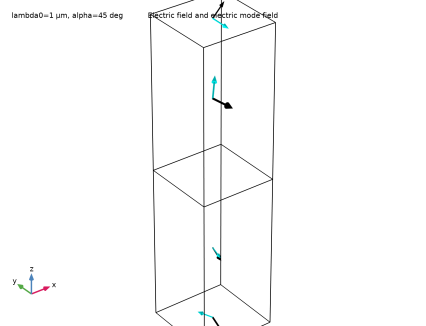
In the Settings window for Arrow Volume, click Replace Expression in the upper-right corner of the Expression section. From the menu, choose Component 1 (comp1) > Electromagnetic Waves, Frequency Domain > Energy and power > ewfd.Poavx,...,ewfd.Poavz - Power flow, time average.
3
Locate the Coloring and Style section. From the Color list, choose Black.
Arrow Volume 3
1
In the Model Builder window, under Results > Electric Field Vectors right-click Arrow Volume 1 and choose Duplicate.
2
In the Settings window for Arrow Volume, locate the Data section.
3
From the Dataset list, choose Study 2/Solution 2 (sol2).
4
From the Parameter value (alpha (deg)) list, choose 45.
5
Click Replace Expression in the upper-right corner of the Expression section. From the menu, choose Component 1 (comp1) > Electromagnetic Waves, Frequency Domain 2 > Electric > ewfd2.Ex,ewfd2.Ey,ewfd2.Ez - Electric field.
6
Locate the Coloring and Style section. From the Color list, choose Green.
Arrow Volume 4
1
Right-click Arrow Volume 3 and choose Duplicate.
2
In the Settings window for Arrow Volume, locate the Data section.
3
From the Dataset list, choose Study 3/Solution 3 (sol3).
4
Click Replace Expression in the upper-right corner of the Expression section. From the menu, choose Component 1 (comp1) > Electromagnetic Waves, Frequency Domain 3 > Electric > ewfd3.Ex,ewfd3.Ey,ewfd3.Ez - Electric field.
5
Locate the Coloring and Style section. From the Color list, choose Cyan.
Arrow Surface 1
1
In the Model Builder window, right-click Electric Field Vectors and choose Arrow Surface.
2
In the Settings window for Arrow Surface, click Replace Expression in the upper-right corner of the Expression section. From the menu, choose Component 1 (comp1) > Electromagnetic Waves, Frequency Domain > Ports > Electric mode field amplitudes > ewfd.Eamplx_1,...,ewfd.Eamplz_1 - Electric mode field amplitude, port 1.
3
Locate the Arrow Positioning section. In the Number of arrows text field, type 1.
Selection 1
1
Right-click Arrow Surface 1 and choose Selection.
2
In the Settings window for Selection, locate the Selection section.
3
From the Selection list, choose Port 1.
Arrow Surface 1
1
In the Model Builder window, click Arrow Surface 1.
2
In the Settings window for Arrow Surface, locate the Coloring and Style section.
3
Arrow Surface 2
1
Right-click Results > Electric Field Vectors > Arrow Surface 1 and choose Duplicate.
2
In the Settings window for Arrow Surface, click Replace Expression in the upper-right corner of the Expression section. From the menu, choose Component 1 (comp1) > Electromagnetic Waves, Frequency Domain > Ports > Wave vectors > ewfd.kModex_1,...,ewfd.kModez_1 - Port mode wave vector, port 1.
3
Locate the Coloring and Style section. From the Color list, choose Black.
4
Arrow Surface 3
1
Right-click Arrow Surface 1 and choose Duplicate.
2
In the Settings window for Arrow Surface, locate the Data section.
3
From the Dataset list, choose Study 2/Solution 2 (sol2).
4
From the Parameter value (alpha (deg)) list, choose 45.
5
Locate the Expression section. In the X-component text field, type ewfd2.Eamplx_1.
6
In the Y-component text field, type ewfd2.Eamply_1.
7
In the Z-component text field, type ewfd2.Eamplz_1.
8
Locate the Coloring and Style section. From the Color list, choose Green.
Arrow Surface 4
1
Right-click Arrow Surface 3 and choose Duplicate.
2
In the Settings window for Arrow Surface, locate the Data section.
3
From the Dataset list, choose Study 3/Solution 3 (sol3).
4
Locate the Expression section. In the X-component text field, type ewfd3.Eamplx_1.
5
In the Y-component text field, type ewfd3.Eamply_1.
6
In the Z-component text field, type ewfd3.Eamplz_1.
7
Locate the Coloring and Style section. From the Color list, choose Cyan.
Arrow Surface 5
1
In the Model Builder window, under Results > Electric Field Vectors right-click Arrow Surface 1 and choose Duplicate.
2
In the Settings window for Arrow Surface, locate the Expression section.
3
In the X-component text field, type ewfd.Eamplx_2.
4
In the Y-component text field, type ewfd.Eamply_2.
5
In the Z-component text field, type ewfd.Eamplz_2.
Selection 1
1
In the Model Builder window, expand the Arrow Surface 5 node, then click Selection 1.
2
In the Settings window for Selection, locate the Selection section.
3
From the Selection list, choose Port 2.
Arrow Surface 6
1
In the Model Builder window, under Results > Electric Field Vectors right-click Arrow Surface 2 and choose Duplicate.
2
In the Settings window for Arrow Surface, locate the Expression section.
3
In the X-component text field, type ewfd.kModex_2.
4
In the Y-component text field, type ewfd.kModey_2.
5
In the Z-component text field, type ewfd.kModez_2.
Selection 1
1
In the Model Builder window, expand the Arrow Surface 6 node, then click Selection 1.
2
In the Settings window for Selection, locate the Selection section.
3
From the Selection list, choose Port 2.
Arrow Surface 7
1
In the Model Builder window, under Results > Electric Field Vectors right-click Arrow Surface 5 and choose Duplicate.
2
In the Settings window for Arrow Surface, locate the Data section.
3
From the Dataset list, choose Study 2/Solution 2 (sol2).
4
From the Parameter value (alpha (deg)) list, choose 45.
5
Locate the Expression section. In the X-component text field, type ewfd2.Eamplx_2.
6
In the Y-component text field, type ewfd2.Eamply_2.
7
In the Z-component text field, type ewfd2.Eamplz_2.
8
Locate the Coloring and Style section. From the Color list, choose Green.
Arrow Surface 8
1
Right-click Arrow Surface 7 and choose Duplicate.
2
In the Settings window for Arrow Surface, locate the Data section.
3
From the Dataset list, choose Study 3/Solution 3 (sol3).
4
Locate the Expression section. In the X-component text field, type ewfd3.Eamplx_2.
5
In the Y-component text field, type ewfd3.Eamply_2.
6
In the Z-component text field, type ewfd3.Eamplz_2.
7
Locate the Coloring and Style section. From the Color list, choose Cyan.
Electric Field Vectors
1
In the Model Builder window, click Electric Field Vectors.
2
In the Settings window for 3D Plot Group, locate the Title section.
3
From the Title type list, choose Manual.
4
In the Title text area, type Electric field and electric mode field.
5
In the Electric Field Vectors toolbar, click  Plot.
6
Click the  Zoom Extents button in the Graphics toolbar.
Animation 1
1
In the Electric Field Vectors toolbar, click  Animation and choose Player.
2
In the Settings window for Animation, locate the Animation Editing section.
3
From the Sequence type list, choose Dynamic data extension.
4
Locate the Frames section. In the Number of frames text field, type 25.
5
Locate the Playing section. From the Repeat list, choose Number of iterations.
6
In the Number of iterations text field, type 5.
7
Click the  Play button in the Graphics toolbar.
This animation of the arrow plots shows that the solutions based on the three different physics interfaces are the same. Furthermore, it is clear that the domain fields and the port mode field on the transmission side represent right-handed circularly polarized waves, whereas the mode field for the outgoing wave on the excitation port boundary represents a left-handed circularly polarized wave.
Arrow Surface 1
Finally, add the electric mode field amplitude for the Orthogonal Polarization node at the excitation port boundary, to verify that the Port and the Orthogonal Polarization nodes indeed have orthogonal polarizations.
Arrow Surface 9
1
In the Model Builder window, under Results > Electric Field Vectors right-click Arrow Surface 1 and choose Duplicate.
2
In the Settings window for Arrow Surface, click Replace Expression in the upper-right corner of the Expression section. From the menu, choose Component 1 (comp1) > Electromagnetic Waves, Frequency Domain > Ports > Electric mode field amplitudes > ewfd.Eamplx_3,...,ewfd.Eamplz_3 - Electric mode field amplitude, port 3.
Use the Zoom In button in the Graphics toolbar and the left and right mouse buttons to get a good close up view of the top port boundary with the electric mode field amplitude vectors for the Port and the Orthogonal Polarization nodes.
Animation 1
1
Click the  Play button in the Graphics toolbar.
This animation shows that the mode field amplitudes for the Port (cyan) and the Orthogonal Polarization subnode (red) rotates in opposite directions — left-handed circular polarization for the Port and right-handed circular polarization for the Orthogonal Polarization node.