PDF

Inverse Uncertainty Quantification of Tensile Test
Introduction
This example demonstrates how to perform inverse uncertainty quantification analysis to calibrate Young’s modulus and Poisson’s ratio based on a tensile test. The test measures the radial displacement and the tensile force at specified locations of the solid specimen based on different axial displacements. The test data is generated with synthetic data generated in the model. The posterior distributions of the calibrated Young’s modulus and Poisson’s ratio are computed based on their prior distributions and the test data.
Model Definition
The model runs an inverse uncertainty quantification study using the radial displacement and the tensile force at specified locations of the solid specimen as the quantities of interest. In order to perform the uncertainty quantification analysis, three random variables need to be defined as input parameters. First, the prior knowledge of Young’s modulus and Poisson’s ratio that need to be calibrated. Second, the experimental parameter, the axial displacement, which is the same as the parameter used to generate the test data. The input parameter distributions are set according to the table in Figure 1.
Figure 1: Input-parameter distributions used in inverse uncertainty quantification.
This tutorial begins with the stationary study for generating the tensile test data. In this analysis, the specimen is assumed to have prescribed displacement in the z direction, where the specified displacement is considered as the experimental parameter. The test data is first generated assuming a Young’s modulus value of 200 GPa and a Poisson’s ratio of 0.3. The data is then perturbed with noise generated from a Gaussian distribution using a global evaluation. For details, see the Modeling Instructions section.
The experimental data settings in the UQ study uses the tensile test data as the experiential data table. The data column type is specified according to the table in Figure 2.
Figure 2: Experimental data settings used in inverse uncertainty quantification.
Results and Discussion
The uncertainty quantification study gives the joint probability distribution plot shown in Figure 3, with associated confidence interval information in the calibrated confidence interval table shown in Figure 4. The posterior means of Young’s modulus and Poisson’s ratio are close to their values used to generate the tensile test data. From the joint probability distribution plot, there is no strong correlation between Young’s modulus and Poisson’s ratio.
Figure 3: Joint probability distribution.
Figure 4: Calibrated confidence interval.
Application Library path: Uncertainty_Quantification_Module/Tutorials/tensile_test_uncertainty_quantification
Modeling Instructions
From the File menu, choose New.
New
In the New window, click  Blank Model.
Global Definitions
Parameters 1
1
In the Model Builder window, under Global Definitions click Parameters 1.
2
In the Settings window for Parameters, locate the Parameters section.
3
Geometrical Parameters
1
In the Home toolbar, click  Parameters and choose Add > Parameters.
2
In the Settings window for Parameters, type Geometrical Parameters in the Label text field.
3
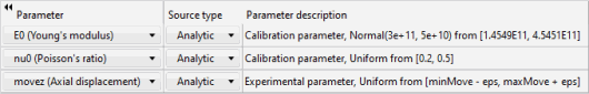
Locate the Parameters section. In the table, enter the following settings:
Add Component
In the Home toolbar, click  Add Component and choose 2D Axisymmetric.
Definitions
Random 1 (rn1)
1
In the Definitions toolbar, click  More Functions and choose Random.
2
In the Settings window for Random, locate the Parameters section.
3
From the Distribution list, choose Normal.
Geometry 1
1
In the Model Builder window, under Component 1 (comp1) click Geometry 1.
2
In the Settings window for Geometry, locate the Units section.
3
From the Length unit list, choose mm.
Rectangle 1 (r1)
1
In the Geometry toolbar, click  Rectangle.
2
In the Settings window for Rectangle, locate the Size and Shape section.
3
In the Width text field, type r1.
4
In the Height text field, type L1/2.
5
Click  Build Selected.
Rectangle 2 (r2)
1
In the Geometry toolbar, click  Rectangle.
2
In the Settings window for Rectangle, locate the Position section.
3
In the z text field, type L1/2.
4
Locate the Size and Shape section. In the Width text field, type r2.
5
In the Height text field, type L2.
6
Click  Build Selected.
7
Click the  Zoom Extents button in the Graphics toolbar.
Circular Arc 1 (ca1)
1
In the Geometry toolbar, click  More Primitives and choose Circular Arc.
2
In the Settings window for Circular Arc, locate the Properties section.
3
From the Specify list, choose Endpoints and radius.
4
Locate the Starting Point section. In the r text field, type r2.
5
In the z text field, type L1/2.
6
Locate the Endpoint section. In the r text field, type r1.
7
In the z text field, type L3.
8
Locate the Radius section. In the Radius text field, type r3.
9
Click  Build Selected.
Convert to Solid 1 (csol1)
1
In the Geometry toolbar, click  Conversions and choose Convert to Solid.
2
In the Settings window for Convert to Solid, locate the Input section.
3
From the Input objects list, choose All objects.
4
Locate the Selections of Resulting Entities section. Select the Resulting objects selection checkbox.
5
Click  Build Selected.
Union 1 (uni1)
1
In the Geometry toolbar, click  Booleans and Partitions and choose Union.
2
In the Settings window for Union, locate the Union section.
3
From the Input objects list, choose Convert to Solid 1.
4
Clear the Keep interior boundaries checkbox.
5
Click to clear the  Activate Selection toggle button for Input objects.
6
Click  Build Selected.
Add Physics
1
In the Home toolbar, click  Add Physics to open the Add Physics window.
2
Go to the Add Physics window.
3
In the tree, select Structural Mechanics > Solid Mechanics (solid).
4
Click the Add to Component 1 button in the window toolbar.
5
In the Home toolbar, click  Add Physics to close the Add Physics window.
Materials
Material 1 (mat1)
1
In the Model Builder window, under Component 1 (comp1) right-click Materials and choose Blank Material.
2
In the Settings window for Material, locate the Material Contents section.
3
Solid Mechanics (solid)
Symmetry Plane 1
In the Physics toolbar, click  Boundaries and choose Symmetry Plane.
Prescribed Displacement 1
In the Physics toolbar, click  Boundaries and choose Prescribed Displacement.
Symmetry Plane 1
1
In the Model Builder window, click Symmetry Plane 1.
2
Prescribed Displacement 1
1
In the Model Builder window, click Prescribed Displacement 1.
2
Definitions
Domain Point Probe 1
1
In the Definitions toolbar, click  Probes and choose Domain Point Probe.
2
In the Settings window for Domain Point Probe, locate the Point Selection section.
3
In row Coordinates, set r to r1.
Point Probe Expression 1 (ppb1)
1
In the Model Builder window, expand the Domain Point Probe 1 node, then click Point Probe Expression 1 (ppb1).
2
In the Settings window for Point Probe Expression, locate the Expression section.
3
In the Expression text field, type -u.
4
From the Table and plot unit list, choose m.
5
In the Variable name text field, type r_change.
Boundary Probe 1 (bnd1)
1
In the Definitions toolbar, click  Probes and choose Boundary Probe.
2
In the Settings window for Boundary Probe, type tensile_force in the Variable name text field.
3
Locate the Probe Type section. From the Type list, choose Integral.
4
Locate the Source Selection section. From the Selection list, choose Manual.
5
6
Locate the Expression section. In the Expression text field, type solid.sz.
Solid Mechanics (solid)
1
Click the  Show More Options button in the Model Builder toolbar.
2
In the Show More Options dialog, select Physics > Advanced Physics Options in the tree.
3
In the tree, select the checkbox for the node Physics > Advanced Physics Options.
4
5
In the Model Builder window, under Component 1 (comp1) click Solid Mechanics (solid).
6
In the Settings window for Solid Mechanics, click to expand the Advanced Settings section.
7
Find the Group ODE variables in solver subsection. Clear the Rigid materials checkbox.
Prescribed Displacement 1
1
In the Model Builder window, under Component 1 (comp1) > Solid Mechanics (solid) click Prescribed Displacement 1.
2
In the Settings window for Prescribed Displacement, locate the Prescribed Displacement section.
3
From the Displacement in z direction list, choose Prescribed.
4
In the u0z text field, type movez.
Add Study
1
In the Home toolbar, click  Add Study to open the Add Study window.
2
Go to the Add Study window.
3
Find the Studies subsection. In the Select Study tree, select General Studies > Stationary.
4
Click the Add Study button in the window toolbar.
Study 1
Step 1: Stationary
1
In the Settings window for Stationary, locate the Study Settings section.
2
Select the Include geometric nonlinearity checkbox.
3
Click to expand the Study Extensions section. Select the Auxiliary sweep checkbox.
4
5
6
In the Study toolbar, click  Compute.
Results
Global Evaluation 1
1
In the Results toolbar, click  Global Evaluation.
2
In the Settings window for Global Evaluation, locate the Expressions section.
3
4
Click  Evaluate.
Add Study
1
Go to the Add Study window.
2
Find the Studies subsection. In the Select Study tree, select General Studies > Stationary.
3
Click the Add Study button in the window toolbar.
4
In the Home toolbar, click  Add Study to close the Add Study window.
Study 2
Uncertainty Quantification
In the Study toolbar, click  More Study Extensions and choose Uncertainty Quantification.
Step 1: Stationary
1
In the Settings window for Stationary, locate the Study Settings section.
2
Select the Include geometric nonlinearity checkbox.
Uncertainty Quantification
1
In the Model Builder window, click Uncertainty Quantification.
2
In the Settings window for Uncertainty Quantification, locate the Uncertainty Quantification Settings section.
3
From the UQ study type list, choose Inverse uncertainty quantification.
4
Locate the Quantities of Interest section. Click  Add.
5
6
7
8
Locate the Uncertainty Quantification Settings section. Find the Surrogate model settings subsection. From the Surrogate model list, choose Adaptive sparse polynomial chaos expansion.
9
Locate the Input Parameters section. Click  Add.
10
11
From the Distribution list, choose Normal(μ,σ).
12
In the Mean text field, type 3e+11.
13
In the Standard deviation text field, type 5e+10.
14
15
16
In the Lower bound text field, type 0.2.
17
In the Upper bound text field, type 0.5.
18
19
20
In the Lower bound text field, type minMove - eps.
21
In the Upper bound text field, type maxMove + eps.
22
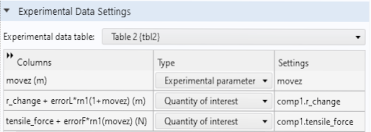
Locate the Experimental Data Settings section. From the Experimental data table list, choose Table 2.
23
24
From the Name list, choose movez.
25
26
From the Name list, choose comp1.r_change.
27
28
From the Name list, choose comp1.tensile_force.
29
In the Study toolbar, click  Compute.
Results
Stress, 3D (solid) 1
Click the  Zoom Extents button in the Graphics toolbar.