|
|
|
|
•
|
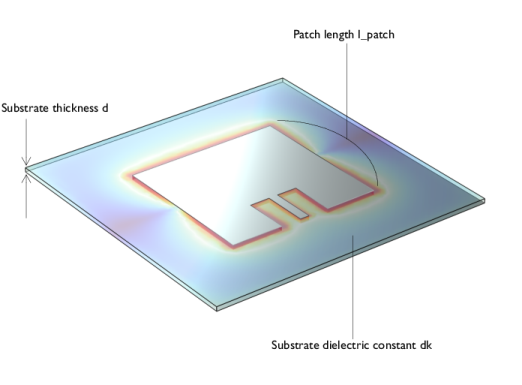
The substrate thickness can vary within about ±7% based on a manufacturer’s data sheet. If the standard deviation (σ) for the thickness is 3.5% of the nominal thickness, then the range specified by d ± 2σ will cover approximately 95.45% of the variations.
|
|
•
|
The tolerance for l_patch is initially based on a scenario using a milling machine with a loosely anchored circuit board. This results in an undesired tolerance of 2σ, 0.520 mm, where σ is 0.005*l_patch. After computing the probability of conditions for this scenario, another reliability analysis is performed assuming non-high-precision PCB fabrication, with an etching tolerance of 0.127 mm (0.005 inches). In this case, σ is set to 0.00125*l_patch, making 2σ approximately equal to 0.127 mm.
|
|
•
|
According to a manufacturer’s data sheet, the dielectric constant (relative permittivity) dk is given as 3.38 ± 0.05 For strict range coverage such as 99.73%, the dielectric constant varies within dk ± 3σ, where σ is 0.005*dk, which equals 0.0169. Therefore, the range corresponds to 3.38 ± 0.0507, that is close to the example value suggested by manufacturers.
|
|
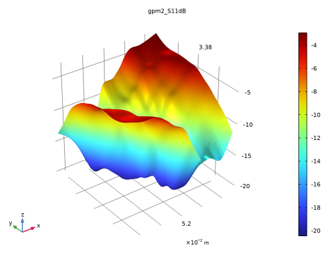
S11 dB shows how much reflection or impedance mismatch at the excited port.
|
|||
|
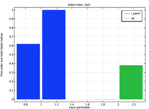
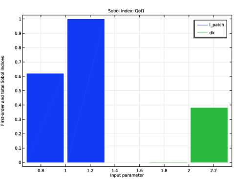
Sobol plot shows the sensitivity of S11 dB to a single parameter variations, and the overall sensitivity contribution including interactions with other parameters.
|
|||
|
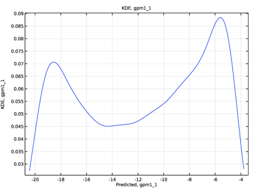
Chance that S11 dB will fall below -10 dB.
|
|||
|
Chance that S11 dB will fall below -10 dB.
|


|
1
|
|
2
|
|
1
|
In the Model Builder window, expand the Component 1 (comp1) > Materials node, then click Substrate (mat2).
|
|
2
|
|
1
|
|
2
|
|
3
|
Click
|
|
5
|
|
7
|
|
8
|
|
9
|
|
10
|
|
11
|
|
12
|
|
13
|
|
14
|
Click
|
|
16
|
|
17
|
|
18
|
|
19
|
|
20
|
|
21
|
|
22
|
|
23
|
Click
|
|
25
|
|
26
|
|
27
|
|
28
|
|
29
|
|
30
|
|
31
|
|
32
|
|
1
|
|
2
|
|
1
|
In the Model Builder window, under Study 4, UQ Sensitivity Analysis click Uncertainty Quantification.
|
|
2
|
|
4
|
Click
|
|
1
|
In the Model Builder window, under Results > Uncertainty Quantification Graph 1 click Sobol Index, QoI1.
 |
|
1
|
|
2
|
|
1
|
In the Model Builder window, under Study 5, UQ Uncertainty Propagation click Uncertainty Quantification.
|
|
2
|
In the Settings window for Uncertainty Quantification, locate the Uncertainty Quantification Settings section.
|
|
3
|
|
1
|
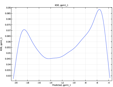
In the Model Builder window, under Results > Uncertainty Quantification Graph 2 click Kernel Density Estimation, gpm1_1.
 |
|
1
|
|
2
|
In the Settings window for Study, type Study 6, UQ Reliability Analysis for Milling with Loose Anchoring in the Label text field.
|
|
1
|
In the Model Builder window, under Study 6, UQ Reliability Analysis for Milling with Loose Anchoring click Uncertainty Quantification.
|
|
2
|
In the Settings window for Uncertainty Quantification, locate the Uncertainty Quantification Settings section.
|
|
3
|
|
4
|
Locate the Quantities of Interest section. In the table, enter the following settings:
|
|
5
|
Locate the Surrogate-Based Response Surface section. In the table, enter the following settings:
|
|
1
|
In the Model Builder window, expand the Results > Tables > Reliability Analysis node, then click Study 6, UQ Reliability Analysis for Milling with Loose Anchoring > Uncertainty Quantification.
|
|
2
|
In the Settings window for Uncertainty Quantification, locate the Surrogate-Based Response Surface section.
|
|
3
|
Click Response Surface in the upper-right corner of the section.
|
|
1
|
|
1
|
|
2
|
In the Settings window for Study, type Study 7, UQ Reliability Analysis for Non-High-Precision PCB Etching in the Label text field.
|
|
1
|
In the Model Builder window, under Study 7, UQ Reliability Analysis for Non-High-Precision PCB Etching click Uncertainty Quantification.
|
|
2
|
In the Settings window for Uncertainty Quantification, locate the Uncertainty Quantification Settings section.
|
|
3
|
|
4
|
Locate the Quantities of Interest section. In the table, enter the following settings:
|
|
5
|
Locate the Input Parameters section. In the table, click to select the cell at row number 1 and column number 3.
|
|
6
|
|
7
|
|
8
|
|
9
|
Locate the Surrogate-Based Response Surface section. In the table, enter the following settings:
|
|
1
|