|
|
|
|
1
|
|
2
|
Go to the Add Study window.
|
|
3
|
Find the Studies subsection. In the Select Study tree, select Preset Studies for Selected Physics Interfaces > Stationary.
|
|
4
|
Click the Add Study button in the window toolbar.
|
|
5
|
|
1
|
|
1
|
|
2
|
|
3
|
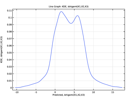
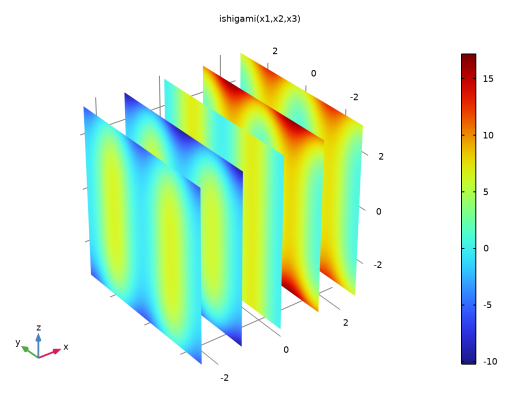
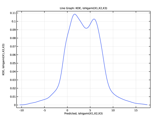
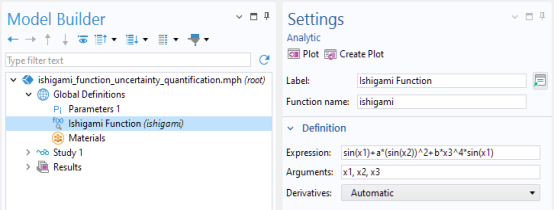
Locate the Definition section. In the Expression text field, type sin(x1)+a*(sin(x2))^2+b*x3^4*sin(x1).
|
|
4
|
|
5
|
|
6
|
Locate the Plot Parameters section. In the table, enter the following settings:
|
|
7
|
Click
|
|
1
|
|
2
|
|
3
|
Click
|
|
5
|
|
7
|
|
8
|
|
10
|
|
11
|
|
13
|
|
14
|
|
15
|
|
1
|
|
2
|
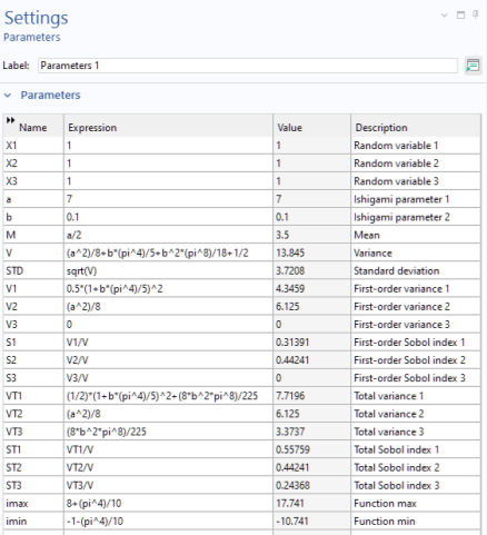
In the Settings window for Uncertainty Quantification, locate the Uncertainty Quantification Settings section.
|
|
3
|
|
1
|
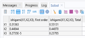
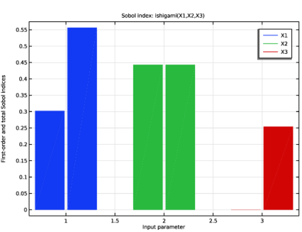
In the Model Builder window, under Results > Uncertainty Quantification Graph 1 click Sobol Index, QoI1.
 |
|
1
|
|
2
|
In the Settings window for Uncertainty Quantification, locate the Uncertainty Quantification Settings section.
|
|
3
|
Find the Surrogate model settings subsection. From the Surrogate model list, choose Adaptive sparse polynomial chaos expansion.
|
|
4
|