PDF

Bow-Tie Antenna Optimization
Introduction
A bow tie antenna patterned on a dielectric substrate is optimized by adjusting the length of the arms and the flare angle to reduce the magnitude of S11, reflection coefficient. The two geometric dimensions used as design variables directly control the antenna’s size and shape, and also affect the dimensions of the dielectric substrate. The Efficient Global Optimization (EGO) method is employed to improve the objective function, |S11| and a reliability analysis is conducted to assess the robustness of the optimized design with respect to design parameter variations.
Figure 1: Outline of a bow tie antenna on a dielectric substrate.
Model Definition
The bow tie antenna model consists of a rectangular dielectric substrate with two triangular metal patterns on top, as shown in Figure 1. The flare angle and the height of the arms define the antenna’s shape. To keep the substrate size minimal, it is defined to extend 2 mm beyond the antenna pattern. A lumped port excitation is applied to a small rectangular face between the antenna arms, simulating a 50 Ω transmission line feed.
The two design variables, flare angle and arm height, control a total of four dimensions in the model. The height and width of the rectangular dielectric substrate are slightly larger than the antenna profile. Consequently, the two design variables directly influence two other geometric dimensions in the model, which in turn affect the antenna characteristics.
Efficient Global Optimization
The reflection coefficient, |S11|, is minimized using the Efficient Global Optimization (EGO) method. EGO is designed for optimizing complex, costly-to-evaluate functions by employing surrogate models, such as Gaussian Processes. It iteratively refines these models to predict the objective function, |S11| and uses the Monte Carlo method to maximize the acquisition function to decide the next point to evaluate, effectively analyzing problems where the function evaluation are expensive. By improving the surrogate model and sampling efficiently, EGO finds optimal solutions with a limited number of evaluations.
Due to the nonanalytic nature of the objective function, derivatives cannot be computed analytically with respect to the design variables. Additionally, the design parameters introduce significant geometric changes to the computational domains and can generate multiple minima during optimization. These factors necessitate the use of the EGO, a gradient-free optimization method, suitable as it does not require gradient information and helps avoid local minima. Using this approximate gradient information, the objective function is iteratively improved until the design variables converge within the desired tolerance.
Reliability Analysis
The Gaussian Process surrogate model used for the EGO is reused to perform a reliability analysis as part of uncertainty quantification with design parameter variations. The reliability analysis determines the probability that a specific condition related to the Quantity of Interest (QoI) will be satisfied. It evaluates the likelihood of meeting a predefined criterion based on the QoI. For example, it calculates the probability that the S-parameter is below 10 dB, helping to assess the reliability of meeting performance specifications. The S-parameter S11 in dB indicates the level of reflection or impedance mismatch at the antenna input port. The threshold of 10 dB is conventionally used, and when it is lower than 10 dB, the reflection due to the impedance mismatch is considered acceptable.
Note: In addition to the RF Module, this example requires the Optimization Module.
Results and Discussion
The model is analyzed at a single frequency of 30 GHz. The optimizer adjusts the flare angle and arm height to reduce the reflection coefficient. For the initial, unoptimized design, |S11| is approximately 0.645, while for the optimized design, |S11| is around 0.2, which corresponds 14 dB on the dB scale. The optimized values for the height and flare angle are close to 1.429 mm and 30°, respectively.
|S11|
Figure 2: Logarithmic plot of the electric field norm after optimization.
The reliability analysis determines the probability that S11 is below 10 dB. The table titled Probability for Conditions in the Reliability Analysis group provides a value of approximately 0.89. This indicates that, under the given design parameter variations, there is about a 89% chance that S11 will be less than 10 dB, which is considered acceptable. The results suggests that, to achieve more robust performance of the printed antenna in the millimeter-wave range, high-precision etching is necessary rather than the conventional standard etching used for typical low-frequency printed circuit boards (PCBs).
Application Library path: Uncertainty_Quantification_Module/Tutorials/bowtie_antenna_optimization
Modeling Instructions
From the File menu, choose New.
New
In the New window, click  Model Wizard.
Model Wizard
1
In the Model Wizard window, click  3D.
2
In the Select Physics tree, select Radio Frequency > Electromagnetic Waves, Frequency Domain (emw).
3
Click Add.
4
Click  Study.
5
In the Select Study tree, select General Studies > Frequency Domain.
6
Global Definitions
Parameters 1
1
In the Model Builder window, under Global Definitions click Parameters 1.
2
In the Settings window for Parameters, locate the Parameters section.
3
Study 1
Step 1: Frequency Domain
1
In the Model Builder window, under Study 1 click Step 1: Frequency Domain.
2
In the Settings window for Frequency Domain, locate the Study Settings section.
3
In the Frequencies text field, type f0.
Geometry 1
1
In the Model Builder window, under Component 1 (comp1) click Geometry 1.
2
In the Settings window for Geometry, locate the Units section.
3
From the Length unit list, choose mm.
Work Plane 1 (wp1)
1
In the Geometry toolbar, click  Work Plane.
2
In the Settings window for Work Plane, locate the Unite Objects section.
3
Clear the Unite objects checkbox.
Work Plane 1 (wp1) > Plane Geometry
In the Model Builder window, click Plane Geometry.
Work Plane 1 (wp1) > Square 1 (sq1)
1
In the Work Plane toolbar, click  Square.
2
In the Settings window for Square, locate the Size section.
3
In the Side length text field, type L0.
4
Locate the Rotation Angle section. In the Rotation text field, type theta/2.
Work Plane 1 (wp1) > Mirror 1 (mir1)
1
In the Work Plane toolbar, click  Transforms and choose Mirror.
2
3
In the Settings window for Mirror, locate the Input section.
4
Select the Keep input objects checkbox.
5
Click  Build Selected.
Work Plane 1 (wp1) > Rectangle 1 (r1)
1
In the Work Plane toolbar, click  Rectangle.
2
In the Settings window for Rectangle, locate the Size and Shape section.
3
In the Width text field, type L0.
4
In the Height text field, type h0.
5
Locate the Position section. From the Base list, choose Center.
6
In the yw text field, type h0/2.
7
Click  Build Selected.
8
Click the  Zoom Extents button in the Graphics toolbar.
Work Plane 1 (wp1) > Intersection 1 (int1)
1
In the Work Plane toolbar, click  Booleans and Partitions and choose Intersection.
2
Click the  Select All button in the Graphics toolbar.
3
In the Settings window for Intersection, click  Build Selected.
4
Click the  Zoom Extents button in the Graphics toolbar.
Work Plane 1 (wp1) > Mirror 2 (mir2)
1
In the Work Plane toolbar, click  Transforms and choose Mirror.
2
3
In the Settings window for Mirror, locate the Normal Vector to Line of Reflection section.
4
In the xw text field, type 0.
5
In the yw text field, type 1.
6
Locate the Input section. Select the Keep input objects checkbox.
7
Click  Build Selected.
8
Click the  Zoom Extents button in the Graphics toolbar.
9
Click the  Zoom Extents button in the Graphics toolbar.
Work Plane 1 (wp1) > Rectangle 2 (r2)
1
In the Work Plane toolbar, click  Rectangle.
2
In the Settings window for Rectangle, locate the Size and Shape section.
3
In the Width text field, type tan(theta/2)*Gap.
4
In the Height text field, type Gap.
5
Locate the Position section. From the Base list, choose Center.
Work Plane 1 (wp1) > Rectangle 3 (r3)
1
In the Work Plane toolbar, click  Rectangle.
2
In the Settings window for Rectangle, locate the Size and Shape section.
3
In the Width text field, type 2*h0*tan(theta/2)+2*Padding.
4
In the Height text field, type 2*h0+2*Padding.
5
Locate the Position section. From the Base list, choose Center.
6
Click  Build Selected.
Extrude 1 (ext1)
1
In the Model Builder window, right-click Geometry 1 and choose Extrude.
2
In the Settings window for Extrude, locate the General section.
3
Click the  Clear Selection button for Input objects.
4
Select the object wp1.r3 only.
5
Locate the Distances section. In the table, enter the following settings:
6
Select the Reverse direction checkbox.
7
Click  Build Selected.
8
Click the  Wireframe Rendering button in the Graphics toolbar.
Sphere 1 (sph1)
1
In the Geometry toolbar, click  Sphere.
2
In the Settings window for Sphere, locate the Size section.
3
In the Radius text field, type 0.75*L0.
4
Click to expand the Layers section. In the table, enter the following settings:
5
Click  Build All Objects.
Definitions
Perfectly Matched Layer 1 (pml1)
1
In the Definitions toolbar, click  Perfectly Matched Layer.
2
3
In the Settings window for Perfectly Matched Layer, locate the Geometry section.
4
From the Type list, choose Spherical.
Add Material from Library
In the Home toolbar, click  Windows and choose Add Material from Library.
Add Material
1
Go to the Add Material window.
2
In the tree, select Built-in > Air.
3
Click the Add to Component button in the window toolbar.
4
In the tree, select Built-in > FR4 (Circuit Board).
5
Click the Add to Component button in the window toolbar.
6
In the Home toolbar, click  Add Material to close the Add Material window.
Materials
FR4 (Circuit Board) (mat2)
Select Domain 6 only.
Electromagnetic Waves, Frequency Domain (emw)
Perfect Electric Conductor 2
1
In the Physics toolbar, click  Boundaries and choose Perfect Electric Conductor.
2
Lumped Port 1
1
In the Physics toolbar, click  Boundaries and choose Lumped Port.
2
Far-Field Domain 1
1
In the Physics toolbar, click  Domains and choose Far-Field Domain.
2
Click the  Zoom Extents button in the Graphics toolbar.
Definitions
Hide for Physics 1
1
In the Model Builder window, right-click View 1 and choose Hide for Physics.
2
In the Settings window for Hide for Physics, locate the Geometric Entity Selection section.
3
From the Geometric entity level list, choose Boundary.
4
Mesh 1
1
In the Model Builder window, under Component 1 (comp1) right-click Mesh 1 and choose Build All.
2
Click the  Zoom In button in the Graphics toolbar.
Study 1
Parameter Optimization
1
In the Study toolbar, click  Optimization and choose Parameter Optimization.
2
In the Settings window for Parameter Optimization, locate the Optimization Solver section.
3
From the Method list, choose EGO.
4
Click to expand the Gaussian Process Function section. Find the Acquisition function settings subsection. From the Optimization method for acquisition function list, choose Monte Carlo.
5
In the Surrogate evaluations for optimization text field, type 1e6.
6
Locate the Objective Function section. In the table, enter the following settings:
7
Locate the Control Parameters section. Click  Add twice.
8
9
In the Study toolbar, click  Compute.
Results
Multislice 1
1
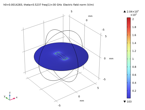
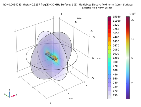
In the Model Builder window, expand the Results > Electric Field (emw) node, then click Multislice 1.
2
In the Settings window for Multislice, locate the Multiplane Data section.
3
Find the X-planes subsection. In the Planes text field, type 0.
4
Find the Y-planes subsection. In the Planes text field, type 0.
5
In the Electric Field (emw) toolbar, click  Plot.
6
Click the  Zoom Extents button in the Graphics toolbar.
Electric Field, Logarithmic (emw)
In the Model Builder window, under Results click Electric Field, Logarithmic (emw).
2D Far Field (emw)
In the Model Builder window, click 2D Far Field (emw).
3D Far Field, Gain (emw)
In the Model Builder window, click 3D Far Field, Gain (emw).
Global Evaluation 2
1
In the Results toolbar, click  Global Evaluation.
2
In the Settings window for Global Evaluation, locate the Expressions section.
3
4
Click  Evaluate.
The Gaussian Process 1 surrogate model used for the EGO can be reused to conduct a reliability analysis as part of uncertainty quantification with design parameter variations.
Add Study
1
In the Home toolbar, click  Add Study to open the Add Study window.
2
Go to the Add Study window.
3
Find the Studies subsection. In the Select Study tree, select General Studies > Frequency Domain.
4
Click the Add Study button in the window toolbar.
5
In the Home toolbar, click  Add Study to close the Add Study window.
Study 2
Step 1: Frequency Domain
1
In the Settings window for Frequency Domain, locate the Study Settings section.
2
In the Frequencies text field, type f0.
3
In the Model Builder window, click Study 2.
4
In the Settings window for Study, locate the Study Settings section.
5
Clear the Generate default plots checkbox.
Uncertainty Quantification
1
In the Study toolbar, click  More Study Extensions and choose Uncertainty Quantification.
2
In the Settings window for Uncertainty Quantification, locate the Uncertainty Quantification Settings section.
3
From the UQ study type list, choose Reliability analysis, EGRA.
4
Find the Surrogate model settings subsection. From the Gaussian process function list, choose Gaussian Process 1 (gpm1_1).
5
From the Compute action list, choose Improve and analyze.
6
Locate the Quantities of Interest section. Click  Add.
7
The given threshold expression will calculate the probability that S11 will fall below -10 dB.
8
Locate the Input Parameters section. Click  Add.
9
10
11
From the Distribution list, choose Normal(μ,σ).
12
In the Mean text field, type 1.4295[mm].
Use the optimized value of the height h0 for the Mean.
13
In the Standard deviation text field, type 1.4295*0.045[mm].
The standard deviation is defined as above to ensure 2σ is close to the non-high-precision etching tolerance of 0.127 mm.
14
From the CDF-Lower list, choose Manual.
15
In the Lower bound text field, type 1.4295[mm]-2*1.4295[mm]*0.045.
16
From the CDF-Upper list, choose Manual.
17
In the Upper bound text field, type 1.4295[mm]+2*1.4295[mm]*0.045.
The range specified by h0±2σ will cover approximately 95.45% of the variations.
18
19
20
21
From the Distribution list, choose Normal(μ,σ).
22
In the Mean text field, type 30[deg].
23
In the Standard deviation text field, type 30[deg]*0.045.
24
From the CDF-Lower list, choose Manual.
25
In the Lower bound text field, type 30[deg]-2*30[deg]*0.045.
26
From the CDF-Upper list, choose Manual.
27
In the Upper bound text field, type 30[deg]+2*30[deg]*0.045.
28
Locate the Surrogate-Based Response Surface section. In the table, enter the following settings:
Uncertainty Quantification 1
In the Study toolbar, click  Compute.
Results
In the Model Builder window, expand the Results > Tables node.
Table 5
The Probability for Conditions table under the Reliability Analysis 1 group shows a value of approximately 0.89. This implies that, under the given conditions — representing a non-high-precision PCB etching tolerance — there is roughly a 89% chance that S11 will fall below -10 dB.