PDF

Variably Saturated Flow
Introduction
This example uses the Richards’ Equation interface to assess how well geophysical irrigation sensors detect the true level of fluid saturation in variably saturated soils. Andrew Hinnell, Alex Furman, and Ty Ferre from the Department of Hydrology and Water Resources at the University of Arizona brought the example to us. They originally worked out the problem in COMSOL Multiphysics’ PDE interfaces, but this discussion shares their elegant model reformulated in the Richards’ Equation interface.
A major challenge when characterizing fluid movement in variably saturated porous media lies primarily in the need to describe how the capacity to transmit and store fluids changes as fluids enter and fill the pore spaces. Experimental data for these properties are difficult to obtain. Moreover, the properties that change value as the soil saturates happen to be equation coefficients, which makes the mathematics notoriously nonlinear. The Richards’ Equation interface provides interfaces that automate the van Genuchten (Ref. 1) as well as the Brooks and Corey (Ref. 2) relationships for fluid retention and material properties that vary with the solution.
Figure 1: A variably saturated porous medium.
This example uses the model of Hinnell, Furman, and Ferre to characterize how the distribution of water changes around three impermeable sensors inserted into two different blocks of uniform soil partially saturated with water. The question for the model to address is this: Does the saturation localized around the sensor give a valid picture of the saturation within the total block?
This example demonstrates how to use the Richards’ Equation interface including the van Genuchten (Ref. 1) as well as the Brooks and Corey (Ref. 2) retention models.
Model Definition
The problem setup is as follows. Two homogeneous columns of soil, each 2 m-by- 2 m on a face, are partially saturated with water. A plot of the hydraulic properties of the first soil (Soil Type 1) fits the van Genuchten retention and permeability formulas. The other soil (Soil Type 2) has material properties that suit the Brooks and Corey formulas. Within each soil column are three impermeable rods, each with a 0.1 m radius. The rods are spaced at 0.5 m increments so they run horizontally down the centerline of each block; see Figure 2. Just after the rods are emplaced, the pressure head is still uniform, but water begins to move vertically downward in steady drainage. Because all vertical slices down a block are identical, you can model a 2D cross section and observe the changes in the flow field for 900 s or 15 minutes.
Figure 2: Soil block with three rods. The shaded plane represents a vertical cross section.
Governing Equation
Richards’ equation describes the unsaturated-saturated flow of water in the soils. In this problem you can only use Richards’ equation for the water since the air in the soil is supposed to be at atmospheric pressure. The governing equation for the model is
Pressure head, Hp (m), is the dependent variable. C denotes specific moisture capacity (), Se is the effective saturation, S is a storage coefficient (m1), t is time, K denotes the hydraulic conductivity (m/s), and D is the coordinate (for example x, y, or z) for the vertical elevation (m). The equation does not show the volumetric fraction of water, θ, which is a constitutive relation that depends on Hp. Nonlinearities appear because C, Se, and K change with Hp and θ.
The first term in the equation explains that fluid storage can change with time during both unsaturated and saturated conditions. When the soil is unsaturated, the pores fill with (or drain) water. After the pore spaces completely fill, there is slight compression of the fluid and the pore space. The specific moisture capacity C = ∂θ/∂Hp describes the change in fluid volume fraction θ with pressure head. The storage coefficient addresses storage changes due to compression and expansion of the pore spaces and the water when the soil is fully wet. To model the storage coefficient, this example uses the specific storage option, which sets S = ρfgp + θχf). Here, ρf is the fluid density (kg/m3), g is the acceleration of gravity, while χp and χf are the compressibilities of the solid particles and fluid, respectively (m·s2/kg).
The van Genuchten and the Brooks and Corey formulas that describe the change in C, Se, K, and θ with Hp require data for the saturated and liquid volume fractions, θs and θr, as well as for other constants α, n, m, and l, which specify a particular type of medium. With the van Genuchten equations that follow, you consider the soil as being saturated when fluid pressure is atmospheric (that is, Hp = 0). With the Brooks and Corey approach, an air-entry pressure distinguishes saturated (Hp > −1/α) and unsaturated (Hp < −1/α) soil. For the detailed formulas, see the section Retention and Permeability Relationships in the Subsurface Flow Module User’s Guide.
To find a unique solution to this problem, you must specify initial and boundary conditions. Initially, the column has uniform pressure head of Hp0. No flow conditions are applied to the rings and to the sides. At the surface and bottom of the geometry the pressure head Hp0is specified.
Model Data
The following table gives the data needed to complete the two example problems:
ρf
χp
m·s2/kg
10-8
10-8
χf
m·s2/kg
Ks
θs
θr
α
m-1
Hp0
Hp0
Results and Discussion
Figure 3 and Figure 4 are solutions to the Richards’ equation problem of Prof. Ty Ferre, Andrew Hinnell, and Alex Furman from the University of Arizona’s Department of Hydrology and Water Resources. Each figure gives results for similar variably saturated flow problem posed for different soil types. Each snapshot shows effective fluid saturation (surface plot), pressure head (contours), and fluid velocities (arrows). The flow field varies around the rods but remains largely uniform over the remainder of each block.
Figure 3: Solution for effective saturation (surface plot), pressure head (contours), and velocity (arrows) at 15 minutes for Soil Type 1 (van Genuchten).
Figure 4: Solution for effective saturation (surface plot), pressure head (contours), and velocity (arrows) at 15 minutes for Soil Type 2 (Brooks and Corey).
Figure 5 shows the effective saturation evolving over time at the rod-soil boundary. The intervals (180°, 0°) and (0°, 180°) for the angular coordinate along the horizontal axis correspond to the boundary’s lower and upper halves, respectively. In the figure, the solid lines denote the solution for Soil Type 1, and the dashed lines correspond to Soil Type 2. The soil is wetter just above the rods than below them.
Figure 5: Effective saturation around the center rod in Soil Type 1 (solid lines) and Soil Type 2 (dashed lines).
Figure 6 compares the average fluid saturations at the rod boundary with the average within the two blocks of soil. The range of effective saturation estimates at the rod boundary appears as a scatter plot for different time steps. The solid line is the average of the effective saturation at the rod boundary. The dashed line is the average of effective saturation for the soil. Clearly the average effective saturation at the rods increases with time, but the average for the soil does not change. While the effects shown here are more pronounced in Soil Type 1 than Soil Type 2, the results call to question whether the sensors can accurately assess soil moisture if kept in situ for long times.
Figure 6: Average effective saturation at sensor circumference and overall soil block for Soil Type 1 (blue) and Soil Type 2 (green). Also shown is the range of effective saturation at the rod circumference for Soil Type 1 (circles) and Soil Type 2 (squares).
The results can also be displayed in 3D using an extrusion dataset. As an example, the effective saturation is plotted in slices within a 3D domain in Figure 7 and Figure 8.
Figure 7: Slice plot of the effective saturation and streamlines of the velocity at 15 minutes for Soil Type 1 (van Genuchten), displayed within a 3D domain.
Figure 8: Slice plot of the effective saturation and streamlines of the velocity at 15 minutes for Soil Type 2(Brooks and Corey), displayed within a 3D domain.
References
1. M.Th. van Genuchten, “A Closed-form Equation for Predicting the Hydraulic of Conductivity of Unsaturated Soils,” Soil Sci. Soc. Am. J., vol. 44, pp. 892–898, 1980.
2. R.H. Brooks and A.T. Corey, “Properties of Porous Media Affecting Fluid Flow,” J. Irrig. Drainage Div., ASCE Proc, vol. 72 (IR2), pp. 61–88, 1966.
Application Library path: Subsurface_Flow_Module/Fluid_Flow/variably_saturated_flow
Modeling Instructions
From the File menu, choose New.
New
In the New window, click  Model Wizard.
Model Wizard
1
In the Model Wizard window, click  2D.
2
In the Select Physics tree, select Fluid Flow > Porous Media and Subsurface Flow > Richards’ Equation (dl).
3
Click Add.
4
Click  Study.
5
In the Select Study tree, select General Studies > Time Dependent.
6
Geometry 1
Square 1 (sq1)
1
In the Geometry toolbar, click  Square.
2
In the Settings window for Square, locate the Size section.
3
In the Side length text field, type 2.
4
Locate the Position section. From the Base list, choose Center.
Circle 1 (c1)
1
In the Geometry toolbar, click  Circle.
2
In the Settings window for Circle, locate the Size and Shape section.
3
In the Radius text field, type 0.1.
4
Locate the Position section. In the x text field, type -0.5.
Array 1 (arr1)
1
In the Geometry toolbar, click  Transforms and choose Array.
2
3
In the Settings window for Array, locate the Size section.
4
In the x size text field, type 3.
5
Locate the Displacement section. In the x text field, type 0.5.
Difference 1 (dif1)
1
In the Geometry toolbar, click  Booleans and Partitions and choose Difference.
2
Select the object sq1 only, to add it to the Objects to add list.
3
In the Settings window for Difference, locate the Difference section.
4
Click to select the  Activate Selection toggle button for Objects to subtract.
5
Select the objects arr1(1,1), arr1(2,1), and arr1(3,1) only.
6
Click  Build All Objects.
Definitions
Next, create the selection to simplify the evaluation of the results.
Rod
1
In the Definitions toolbar, click  Explicit.
2
In the Settings window for Explicit, type Rod in the Label text field.
3
Locate the Input Entities section. From the Geometric entity level list, choose Boundary.
4
5
Select the Group by continuous tangent checkbox.
To investigate the two different retention models, it is useful to work with parameter cases. First, load a set of parameters and create two different parameter sets.
Global Definitions
Parameters 1
1
In the Model Builder window, under Global Definitions click Parameters 1.
2
In the Settings window for Parameters, locate the Parameters section.
3
Click  Load from File.
4
5
In the Home toolbar, click  Parameter Case.
6
In the Settings window for Case, type Case 1: van Genuchten in the Label text field.
7
In the Home toolbar, click  Parameter Case.
8
In the Settings window for Case, type Case 2: Brooks and Corey in the Label text field.
9
Locate the Parameters section. In the table, enter the following settings:
Continue with setting up the physics using the parameters.
Richards’ Equation (dl)
Fluid 1
1
In the Model Builder window, under Component 1 (comp1) > Richards’ Equation (dl) > Unsaturated Porous Medium 1 click Fluid 1.
2
In the Settings window for Fluid, locate the Fluid Properties section.
3
From the Fluid type list, choose Compressible, linearized.
4
From the ρref list, choose User defined. In the associated text field, type rho.
5
From the χf list, choose User defined. In the associated text field, type chi_f.
Porous Matrix 1
1
In the Model Builder window, click Porous Matrix 1.
2
In the Settings window for Porous Matrix, locate the Matrix Properties section.
3
From the εp list, choose User defined. In the associated text field, type poro.
4
In the χp text field, type chi_p.
5
From the Permeability model list, choose Hydraulic conductivity.
6
In the Ks text field, type K.
7
Locate the Retention Model section. In the α text field, type alpha.
8
In the l text field, type l.
9
In the n text field, type n.
10
In the θr text field, type theta_r.
Unsaturated Porous Medium (van Genuchten)
1
In the Model Builder window, under Component 1 (comp1) > Richards’ Equation (dl) click Unsaturated Porous Medium 1.
2
In the Settings window for Unsaturated Porous Medium, type Unsaturated Porous Medium (van Genuchten) in the Label text field.
Unsaturated Porous Medium (Brooks and Corey)
1
Right-click Unsaturated Porous Medium (van Genuchten) and choose Duplicate.
2
In the Settings window for Unsaturated Porous Medium, type Unsaturated Porous Medium (Brooks and Corey) in the Label text field.
Porous Matrix 1
1
In the Model Builder window, expand the Unsaturated Porous Medium (Brooks and Corey) node, then click Porous Matrix 1.
2
In the Settings window for Porous Matrix, locate the Retention Model section.
3
From the Retention model list, choose Brooks and Corey.
Initial Values 1
1
In the Model Builder window, under Component 1 (comp1) > Richards’ Equation (dl) click Initial Values 1.
2
In the Settings window for Initial Values, locate the Initial Values section.
3
Click the Pressure head button.
4
In the Hp text field, type Hp0.
Pressure Head 1
1
In the Physics toolbar, click  Boundaries and choose Pressure Head.
2
3
In the Settings window for Pressure Head, locate the Pressure Head section.
4
In the Hp0 text field, type Hp0.
Mesh 1
Free Triangular 1
In the Mesh toolbar, click  Free Triangular.
Size 1
1
Right-click Free Triangular 1 and choose Size.
2
In the Settings window for Size, locate the Geometric Entity Selection section.
3
From the Geometric entity level list, choose Boundary.
4
5
Locate the Element Size section. Click the Custom button.
6
Locate the Element Size Parameters section.
7
Select the Maximum element size checkbox. In the associated text field, type 0.025.
8
Click  Build All.
Study 1
1
In the Model Builder window, click Study 1.
2
In the Settings window for Study, locate the Study Settings section.
3
Clear the Generate default plots checkbox.
Step 1: Time Dependent
1
In the Model Builder window, under Study 1 click Step 1: Time Dependent.
2
In the Settings window for Time Dependent, locate the Study Settings section.
3
From the Time unit list, choose min.
4
In the Output times text field, type 0 1 5 10 15.
Disable the Unsaturated Porous Medium feature that uses the Brooks and Corey retention model for this study.
5
Locate the Physics and Variables Selection section. Select the Modify model configuration for study step checkbox.
6
In the tree, select Component 1 (comp1) > Richards’ Equation (dl) > Unsaturated Porous Medium (Brooks and Corey).
7
Click  Disable.
Add a Parametric Sweep to run this study for the set of the van Genuchten parameters.
Parametric Sweep
1
In the Study toolbar, click  Parametric Sweep.
2
In the Settings window for Parametric Sweep, locate the Study Settings section.
3
From the Sweep type list, choose Parameter switch.
4
5
6
In the Model Builder window, click Study 1.
7
In the Settings window for Study, type Study 1: van Genuchten in the Label text field.
8
In the Study toolbar, click  Compute.
Results
Follow the steps below to reproduce Figure 3 and Figure 4.
Soil Type 1
1
In the Results toolbar, click  2D Plot Group.
2
In the Settings window for 2D Plot Group, type Soil Type 1 in the Label text field.
Surface 1
1
Right-click Soil Type 1 and choose Surface.
2
In the Settings window for Surface, locate the Expression section.
3
In the Expression text field, type dl.Se.
Arrow Surface 1
In the Model Builder window, right-click Soil Type 1 and choose Arrow Surface.
Contour 1
1
Right-click Soil Type 1 and choose Contour.
2
In the Settings window for Contour, locate the Expression section.
3
In the Expression text field, type dl.Hp.
4
Locate the Coloring and Style section. From the Coloring list, choose Uniform.
5
From the Color list, choose Black.
6
Clear the Color legend checkbox.
7
In the Soil Type 1 toolbar, click  Plot.
Soil Type 1
Set up a new study for the Brooks and Corey parameter set.
Add Study
1
In the Home toolbar, click  Add Study to open the Add Study window.
2
Go to the Add Study window.
3
Find the Studies subsection. In the Select Study tree, select General Studies > Time Dependent.
4
Click the Add Study button in the window toolbar.
5
In the Home toolbar, click  Add Study to close the Add Study window.
Study 2
Step 1: Time Dependent
1
In the Settings window for Time Dependent, locate the Study Settings section.
2
From the Time unit list, choose min.
3
In the Output times text field, type 0 1 5 10 15.
Parametric Sweep
1
In the Study toolbar, click  Parametric Sweep.
2
In the Settings window for Parametric Sweep, locate the Study Settings section.
3
From the Sweep type list, choose Parameter switch.
4
5
6
In the Model Builder window, click Study 2.
7
In the Settings window for Study, type Study 2: Brooks and Corey in the Label text field.
8
Locate the Study Settings section. Clear the Generate default plots checkbox.
9
In the Study toolbar, click  Compute.
Results
Soil Type 2
1
In the Model Builder window, right-click Soil Type 1 and choose Duplicate.
2
In the Settings window for 2D Plot Group, type Soil Type 2 in the Label text field.
3
Locate the Data section. From the Dataset list, choose Study 2: Brooks and Corey/Solution 4 (sol4).
To generate Figure 5, continue with the steps below.
Effective Saturation
1
In the Results toolbar, click  1D Plot Group.
2
In the Settings window for 1D Plot Group, type Effective Saturation in the Label text field.
Line Graph 1
1
Right-click Effective Saturation and choose Line Graph.
2
In the Settings window for Line Graph, locate the Selection section.
3
From the Selection list, choose Rod.
4
Locate the y-Axis Data section. In the Expression text field, type dl.Se.
5
Locate the x-Axis Data section. From the Parameter list, choose Expression.
6
In the Expression text field, type atan2(y,x).
7
From the Unit list, choose °.
The function atan2(y,x) along the circle representing the rod produces unphysical values at one point, because there is 180°=-180°. To avoid this, the data are filtered.
Filter 1
1
Right-click Line Graph 1 and choose Filter.
2
In the Settings window for Filter, locate the Element Selection section.
3
In the Logical expression for inclusion text field, type abs(atan2(y,x))<pi.
4
In the Effective Saturation toolbar, click  Plot.
Line Graph 2
1
In the Model Builder window, under Results > Effective Saturation right-click Line Graph 1 and choose Duplicate.
2
In the Settings window for Line Graph, locate the Data section.
3
From the Dataset list, choose Study 2: Brooks and Corey/Solution 4 (sol4).
4
Click to expand the Coloring and Style section. Find the Line style subsection. From the Line list, choose Dashed.
5
From the Color list, choose Cycle (reset).
Line Graph 1
1
In the Model Builder window, click Line Graph 1.
2
In the Settings window for Line Graph, click to expand the Legends section.
3
Select the Show legends checkbox.
Effective Saturation
1
In the Model Builder window, click Effective Saturation.
2
In the Settings window for 1D Plot Group, click to expand the Title section.
3
From the Title type list, choose Manual.
4
In the Title text area, type Effective Saturation, S<sub>e</sub> (1).
5
Locate the Legend section. From the Position list, choose Upper left.
6
In the Effective Saturation toolbar, click  Plot.
To reproduce Figure 6, start by evaluating the average fluid saturation at the rod boundary and the average within the block.
Surface Average 1
1
In the Results toolbar, click  More Derived Values and choose Average > Surface Average.
2
3
In the Settings window for Surface Average, locate the Expressions section.
4
5
Click  Evaluate.
Access the solution for the Brooks and Corey retention model and evaluate again. An alternative way is to create a second Surface Average node.
6
Locate the Data section. From the Dataset list, choose Study 2: Brooks and Corey/Solution 4 (sol4).
7
Click  Evaluate.
Line Average 2
1
In the Results toolbar, click  More Derived Values and choose Average > Line Average.
2
In the Settings window for Line Average, locate the Selection section.
3
From the Selection list, choose Rod.
4
Locate the Expressions section. In the table, enter the following settings:
5
Clicknext to  Evaluate, then choose New Table.
6
Locate the Data section. From the Dataset list, choose Study 2: Brooks and Corey/Solution 4 (sol4).
7
Click  Evaluate.
Table 2
1
Go to the Table 2 window.
2
Click the Table Graph button in the window toolbar.
Results
Table Graph 1
1
In the Settings window for Table Graph, click to expand the Legends section.
2
Select the Show legends checkbox.
3
From the Legends list, choose Manual.
4
Table Graph 2
1
Right-click Results > 1D Plot Group 4 > Table Graph 1 and choose Duplicate.
2
In the Settings window for Table Graph, locate the Data section.
3
From the Table list, choose Table 1.
4
Locate the Coloring and Style section. Find the Line style subsection. From the Line list, choose Dashed.
5
From the Color list, choose Cycle (reset).
6
Locate the Legends section. In the table, enter the following settings:
Continue by adding the distribution of effective saturation estimates at each output time.
1D Plot Group 4
In the Model Builder window, click 1D Plot Group 4.
Line Graph 1
1
In the 1D Plot Group 4 toolbar, click  Line Graph.
2
In the Settings window for Line Graph, locate the Data section.
3
From the Dataset list, choose Study 1: van Genuchten/Solution 1 (sol1).
4
Locate the Selection section. From the Selection list, choose Rod.
5
Locate the y-Axis Data section. In the Expression text field, type dl.Se.
6
Locate the x-Axis Data section. From the Parameter list, choose Expression.
7
In the Expression text field, type t.
8
From the Unit list, choose min.
9
Locate the Coloring and Style section. From the Color list, choose Blue.
10
From the Width list, choose 2.
11
Find the Line markers subsection. From the Marker list, choose Circle.
12
From the Positioning list, choose Interpolated.
Line Graph 2
1
Right-click Line Graph 1 and choose Duplicate.
2
In the Settings window for Line Graph, locate the Data section.
3
From the Dataset list, choose Study 2: Brooks and Corey/Solution 4 (sol4).
4
Locate the Coloring and Style section. From the Color list, choose Green.
5
Find the Line markers subsection. From the Marker list, choose Square.
Average effective saturation
1
In the Model Builder window, under Results click 1D Plot Group 4.
2
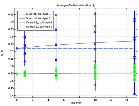
In the Settings window for 1D Plot Group, type Average effective saturation in the Label text field.
3
Locate the Title section. From the Title type list, choose Manual.
4
In the Title text area, type Average effective saturation, S<sub>e</sub>.
5
Locate the Plot Settings section.
6
Select the y-axis label checkbox. In the associated text field, type S<sub>e</sub>(1).
7
Locate the Legend section. From the Position list, choose Upper left.
Extrusion 2D 1
Finally, to reproduce the 3D Plots Figure 7 and Figure 8, follow the steps below.
1
In the Model Builder window, expand the Results > Datasets node.
2
Right-click Results > Datasets and choose More 2D Datasets > Extrusion 2D.
3
In the Settings window for Extrusion 2D, locate the Data section.
4
From the Dataset list, choose Study 1: van Genuchten/Parametric Solutions 1 (sol2).
5
Locate the Extrusion section. Find the Embedding subsection. From the Map plane to list, choose xz-plane.
6
Extrusion 2D 2
1
Right-click Extrusion 2D 1 and choose Duplicate.
2
In the Settings window for Extrusion 2D, locate the Data section.
3
From the Dataset list, choose Study 2: Brooks and Corey/Parametric Solutions 2 (sol5).
3D Plot: Soil Type 1
1
In the Results toolbar, click  3D Plot Group.
2
In the Settings window for 3D Plot Group, type 3D Plot: Soil Type 1 in the Label text field.
Slice 1
1
Right-click 3D Plot: Soil Type 1 and choose Slice.
2
In the Settings window for Slice, click Replace Expression in the upper-right corner of the Expression section. From the menu, choose Component 1 (comp1) > Richards’ Equation > Retention model > dl.Se - Effective saturation - 1.
3
Locate the Plane Data section. From the Plane list, choose zx-planes.
4
In the Planes text field, type 1.
5
Click to expand the Title section. From the Title type list, choose None.
6
In the 3D Plot: Soil Type 1 toolbar, click  Plot.
3D Plot: Soil Type 1
1
In the Model Builder window, click 3D Plot: Soil Type 1.
2
In the Settings window for 3D Plot Group, click to expand the Title section.
3
From the Title type list, choose Custom.
4
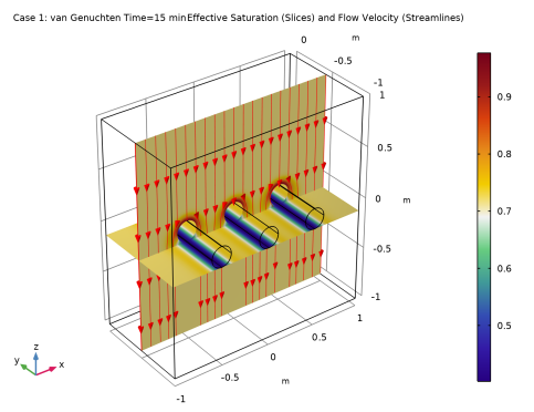
Find the User subsection. In the Suffix text field, type Effective Saturation (Slices) and Flow Velocity (Streamlines).
5
In the 3D Plot: Soil Type 1 toolbar, click  Plot.
Slice 2
1
In the Model Builder window, under Results > 3D Plot: Soil Type 1 right-click Slice 1 and choose Duplicate.
2
In the Settings window for Slice, locate the Plane Data section.
3
From the Plane list, choose xy-planes.
4
In the Planes text field, type 1.
5
Select the Interactive checkbox.
Now use the slider to move the slice to match Figure 7
6
Click to expand the Inherit Style section. From the Plot list, choose Slice 1.
7
In the 3D Plot: Soil Type 1 toolbar, click  Plot.
Streamline 1
1
In the Model Builder window, right-click 3D Plot: Soil Type 1 and choose Streamline.
2
In the Settings window for Streamline, locate the Expression section.
3
In the y-component text field, type 0.
4
In the z-component text field, type dl.v. This has to be done to make sure that the vertical velocity is displayed correctly.
5
Click to expand the Title section. From the Title type list, choose None.
6
Locate the Streamline Positioning section. From the Entry method list, choose Coordinates.
7
In the x text field, type range(-1,0.1,1).
8
In the y text field, type -0.5.
9
In the z text field, type 1.
10
Locate the Coloring and Style section. Find the Point style subsection. From the Type list, choose Arrow.
11
In the 3D Plot: Soil Type 1 toolbar, click  Plot.
12
Click the  Go to Default View button in the Graphics toolbar.
13
Click the  Zoom Extents button in the Graphics toolbar.
3D Plot: Soil Type 2
1
Right-click 3D Plot: Soil Type 1 and choose Duplicate.
2
In the Model Builder window, click 3D Plot: Soil Type 1.1.
3
In the Settings window for 3D Plot Group, type 3D Plot: Soil Type 2 in the Label text field.
4
Locate the Data section. From the Dataset list, choose Extrusion 2D 2.
5
In the 3D Plot: Soil Type 2 toolbar, click  Plot.
6
Click the  Zoom Extents button in the Graphics toolbar.