PDF

Seawater Intrusion in a Coastal Aquifer
Introduction
Seawater intrusion is a significant concern in coastal regions, where the balance between freshwater sources and saltwater infiltration is constantly under threat. This problem is complex because it not only threatens the supply of fresh water but also the quality of groundwater.
This example illustrates how to set up a model for saltwater intrusion in a coastal aquifer when a pumping well is positioned at some distance from the shoreline. The inspiration for this approach arose from the research paper titled “Preferential Flow Enhances Pumping-Induced Saltwater Intrusion in Volcanic Aquifers.” In this research, a range of methods were utilized to replicate the process of saltwater intrusion in a volcanic aquifer distinguished by the presence of highly conductive “lava tubes”, contrasted with other geological formations displaying comparatively lower conductivity levels.
Given the distinctive characteristics of this scenario, where a low-conductivity aquifer intersects with highly conductive tubes, our model incorporates both the homogenized porosity approach as well as the dual porosity approach to capture these conditions.
Model Definition
Figure 1 illustrates the model’s geometry and scenario, with the sea level represented by a hydraulic head condition. The model assumes a consistent rate of freshwater recharge, and the land surface is subjected to precipitation.
Figure 1: Model geometry and conditions.
Freshwater has a density of ρf = 1000 kg/m3, while saltwater has a higher density of ρs = 1025kg/m3. These density differences are essential and are incorporated into the model by considering the transport of salt within the aquifer and utilizing a linearized density relationship:
(1)
Saltwater typically has a salinity of approximately 35% or 35 g/l. In this model, the specific value of cs (maximum salt concentration) is not critical, as all effects are contingent upon the relative salt concentration c. Nonetheless, realistic salt concentration values are utilized by assuming a molar mass of 58.44 g/mol, resulting in cs = 598.9mol/m3.
The transport through the porous aquifer is governed by the conservative formulation of the diffusion–convection equation which also includes dispersion.
(2)
here, Dd and De are the dispersion and diffusion coefficients., εp is the porosity , and on the right hand side Qs denotes the source term. The convective velocity u is calculated using Darcy’s law:
(3)
together with the continuity equation
(4)
Here, K denotes the hydraulic conductivity, g and g are the gravity constant and vector, respectively, while Qm represents a source term. Note that the density ρ is given by Equation 1.
In Ref. 1 the researchers conducted a comparison of different approaches, including a homogenized approach and various heterogeneous approaches to represent diverse facies with distinct conductivities. They specifically set the conductivity for lava tubes to be two orders of magnitude larger than the next highest facies, sparking the idea of investigating a dual porosity approach.
In this example, a homogenized approach is initially considered assuming an anisotropic hydraulic conductivity where horizontal conductivity exceeds vertical conductivity. Then the solution is compared to that of a dual porosity approach.
Dual porosity implies that the flow occurs within the highly conductive area only, namely the lava tubes, which constitute the macroporous part of the system. In contrast, flow within all other facies is stagnant due to their significantly lower conductivity, forming the microporous system. However, these facies can still exchange fluids with the tubes, acting as sources or sinks. Consequently, Equation 3 and Equation 4 are employed for the volume fraction of the macropores (θM). The source term Qm represents the interporosity flow and depends on the pressure difference between the macro- and micropores
(5)
The fluid transfer function αw (s/m2)is influenced by various factors such as the facies structure and characteristics, and it is typically not known with accuracy. A more detailed discussion can be found in Ref. 2. Smaller values of αw indicate longer fluid exchange times. Therefore, when observation periods are sufficiently long and a steady state regime is achieved, the precise value becomes less significant. For the volume fraction of the micropores only an ordinary differential equation (ODE) needs to be solved:
Above equations are incorporated using the Dual Porosity feature within the Darcy’s Law interface. To account for the dual porosity characteristics in salt transport, this is manually integrated by introducing an additional ODE for the micropores:
in conjunction with a mass source term within the transport equation for the macropores (Equation 2) with the mass source being:
Like for the fluid transfer function αw, the mass transfer function αs (1/s) is not known and discussed in Ref. 2.
Results and Discussion
The model is calculated over a duration of one year. Notably, the concentration distribution remains relatively stable after approximately 100 days. The entire year is simulated to account for varying precipitation rates (Figure 2), although it demonstrates that their impact is relatively minor.
Figure 2: Varying precipitation rate over one year.
Figure 3 shows the pressure.
Figure 3: Pressure distribution after one year.
The concentration plot shows the salt concentration for the dual porosity approach. A contour line marks the location of the interface between saltwater and freshwater, where the concentration is 17.5 g/mol, representing half the concentration found in saltwater in the homogenized approach.
Figure 4: Concentration distribution and total concentration flux (arrows) after one year for the dual porosity approach. The black contour line indicates the position of the freshwater–saltwater interface for the homogenized approach.
The outcome of the dual-porosity simulation is that even though the volume fraction of the highly conductive lava tubes is small compared to the aquifer’s low-conductive constituents, they can have a large impact on the saltwater intrusion characteristics. The results show that the dual-porosity approach predict a larger saltwater intrusion as compared to the homogenized approach.
Note that the parameters in this example are chosen arbitrarily. To predict saltwater intrusion in real aquifers it is essential to have good experimental data of the aquifer composition.
References
1. X. Geng and H.A. Michael, “Preferential flow enhances pumping-induced saltwater intrusion in volcanic aquifers,” Water Resour. Res., vol. 56, 2020; doi.org/10.1016/j.jhydrol.2022.127835.
2. T. Vogel, H.H. Gerke, R. Zhang, and M.Th. Van Genuchten, “Modeling flow and transport in a two-dimensional dual-permeability system with spatially variable hydraulic properties,” J. Hydrol., vol.  238, nos. 1–2, pp. 78–89, 2000. doi.org/10.1016/S0022-1694(00)00327-9.
Application Library path: Subsurface_Flow_Module/Solute_Transport/seawater_intrusion
Modeling Instructions
From the File menu, choose New.
New
In the New window, click  Model Wizard.
Model Wizard
1
In the Model Wizard window, click  2D.
2
In the Select Physics tree, select Fluid Flow > Porous Media and Subsurface Flow > Darcy’s Law (dl).
3
Click Add.
4
In the Select Physics tree, select Chemical Species Transport > Transport of Diluted Species in Porous Media (tds).
5
Click Add.
6
Click  Study.
7
In the Select Study tree, select General Studies > Time Dependent.
8
Global Definitions
Start by loading parameters and the geometry sequence into the model.
Parameters 1
1
In the Model Builder window, under Global Definitions click Parameters 1.
2
In the Settings window for Parameters, locate the Parameters section.
3
Click  Load from File.
4
Geometry 1
1
In the Geometry toolbar, click Insert Sequence and choose Insert Sequence.
2
3
In the Geometry toolbar, click  Build All.
Definitions
Next, define a variable for the density to account for density changes due to salt concentration.
Variables 1
1
In the Model Builder window, under Component 1 (comp1) right-click Definitions and choose Variables.
2
In the Settings window for Variables, locate the Variables section.
3
Darcy’s Law (dl)
1
In the Model Builder window, under Component 1 (comp1) click Darcy’s Law (dl).
2
In the Settings window for Darcy’s Law, locate the Gravity Effects section.
3
Select the Include gravity checkbox.
Gravity 1
The sea level is at y = 0m. To accurately account for the influence of gravity effects, the reference position is modified to align with the surface elevation for locations above sea level (y > 0) and is set to 0 for locations below sea level (y < 0).
1
In the Model Builder window, under Component 1 (comp1) > Darcy’s Law (dl) click Gravity 1.
2
In the Settings window for Gravity, locate the Gravity section.
3
Select the Specify reference position checkbox.
4
Specify the rref vector as
Fluid 1
1
In the Model Builder window, under Component 1 (comp1) > Darcy’s Law (dl) > Porous Medium 1 click Fluid 1.
2
In the Settings window for Fluid, locate the Fluid Properties section.
3
From the ρ list, choose User defined. In the associated text field, type rho.
Porous Matrix 1
1
In the Model Builder window, click Porous Matrix 1.
2
In the Settings window for Porous Matrix, locate the Matrix Properties section.
3
From the εp list, choose User defined. In the associated text field, type por.
4
From the Permeability model list, choose Hydraulic conductivity.
5
6
Specify the K matrix as
Initial Values 1
1
In the Model Builder window, under Component 1 (comp1) > Darcy’s Law (dl) click Initial Values 1.
2
In the Settings window for Initial Values, locate the Initial Values section.
3
Click the Hydraulic head button.
Hydraulic Head 1
1
In the Physics toolbar, click  Boundaries and choose Hydraulic Head.
2
3
In the Settings window for Hydraulic Head, locate the Hydraulic Head section.
4
In the H0 text field, type abs(y).
Inlet 1
1
In the Physics toolbar, click  Boundaries and choose Inlet.
2
3
In the Settings window for Inlet, locate the Velocity section.
4
In the U0 text field, type q_in.
Well 1
1
In the Physics toolbar, click  Points and choose Well.
2
3
In the Settings window for Well, locate the Well section.
4
From the Well type list, choose Production.
5
From the Specify list, choose Mass flow.
6
Locate the Mass Flow section. In the M0 text field, type Mwell*dl.rho.
Definitions
Ambient Properties 1 (ampr1)
1
In the Physics toolbar, click  Shared Properties and choose Ambient Properties.
2
In the Settings window for Ambient Properties, locate the Ambient Settings section.
3
From the Ambient data list, choose Meteorological data (ASHRAE 2021).
4
Locate the Location section. Click Set Weather Station.
5
In the Weather Station dialog, type Hono in the text field.
6
In the tree, select Oceania > United States > HONOLULU INTL (911820).
7
Darcy’s Law (dl)
Precipitation 1
1
In the Physics toolbar, click  Boundaries and choose Precipitation.
2
3
In the Settings window for Precipitation, locate the Precipitation section.
4
From the P0 list, choose Ambient precipitation rate (ampr1).
Transport of Diluted Species in Porous Media (tds)
Fluid 1
1
In the Model Builder window, under Component 1 (comp1) > Transport of Diluted Species in Porous Media (tds) > Porous Medium 1 click Fluid 1.
2
In the Settings window for Fluid, locate the Convection section.
3
From the u list, choose Total Darcy velocity field (dl/porous1).
4
Locate the Diffusion section. In the DF,c text field, type D.
Porous Matrix 1
1
In the Model Builder window, click Porous Matrix 1.
2
In the Settings window for Porous Matrix, locate the Matrix Properties section.
3
From the εp list, choose User defined. In the associated text field, type por.
Porous Medium 1
In the Model Builder window, click Porous Medium 1.
Dispersion 1
1
In the Physics toolbar, click  Attributes and choose Dispersion.
2
In the Settings window for Dispersion, locate the Dispersion section.
3
From the Dispersion tensor list, choose Dispersivity.
4
In the αL text field, type 4.
5
In the αT text field, type 0.4.
Concentration 1
1
In the Physics toolbar, click  Boundaries and choose Concentration.
2
3
In the Settings window for Concentration, locate the Concentration section.
4
Select the Species c checkbox.
5
In the c0,c text field, type cs.
Concentration 2
1
In the Physics toolbar, click  Boundaries and choose Concentration.
2
3
In the Settings window for Concentration, locate the Concentration section.
4
Select the Species c checkbox.
Mesh 1
1
In the Model Builder window, under Component 1 (comp1) click Mesh 1.
2
In the Settings window for Mesh, locate the Physics-Controlled Mesh section.
3
From the Element size list, choose Extremely fine.
4
Right-click Component 1 (comp1) > Mesh 1 and choose Edit Physics-Induced Sequence.
Size
1
In the Model Builder window, under Component 1 (comp1) > Mesh 1 click Size.
2
In the Settings window for Size, click to expand the Element Size Parameters section.
3
In the Maximum element size text field, type 5.
4
Click  Build All.
Study 1: Homogenized approach
1
In the Model Builder window, click Study 1.
2
In the Settings window for Study, type Study 1: Homogenized approach in the Label text field.
Step 1: Time Dependent
1
In the Model Builder window, under Study 1: Homogenized approach click Step 1: Time Dependent.
2
In the Settings window for Time Dependent, locate the Study Settings section.
3
From the Time unit list, choose d.
4
In the Output times text field, type range(0,5,365).
5
In the Study toolbar, click  Compute.
By default, plots for the pressure, velocity, and concentration are created automatically. Before examining the results, compute the solution for the dual porosity approach.
Darcy’s Law (dl)
Dual Porosity Medium 1
1
In the Physics toolbar, click  Domains and choose Dual Porosity Medium.
2
3
In the Settings window for Dual Porosity Medium, locate the Interporosity Flow section.
4
In the αw text field, type 1e-3.
Fluid 1
1
In the Model Builder window, click Fluid 1.
2
In the Settings window for Fluid, locate the Fluid Properties section.
3
From the ρ list, choose User defined. In the associated text field, type rho.
4
From the μ list, choose User defined.
Macropores 1
1
In the Model Builder window, click Macropores 1.
2
In the Settings window for Macropores, locate the Matrix Properties section.
3
From the Permeability model list, choose Hydraulic conductivity.
4
Locate the Volume Fraction section. In the θM text field, type theta_M.
5
Locate the Matrix Properties section. From the εp,M list, choose User defined. In the associated text field, type por.
6
From the Permeability model list, choose Power law.
7
In the bPL text field, type bPL.
8
In the nPL text field, type nPL.
Micropores 1
1
In the Model Builder window, click Micropores 1.
2
In the Settings window for Micropores, locate the Matrix Properties section.
3
From the εp,m list, choose User defined. In the associated text field, type por.
Add Physics
1
In the Physics toolbar, click  Add Physics to open the Add Physics window.
2
Go to the Add Physics window.
3
In the tree, select Mathematics > ODE and DAE Interfaces > Domain ODEs and DAEs (dode).
4
Click the Add to Component 1 button in the window toolbar.
5
In the Physics toolbar, click  Add Physics to close the Add Physics window.
Domain ODEs and DAEs (dode)
1
In the Settings window for Domain ODEs and DAEs, locate the Units section.
2
Click  Select Dependent Variable Quantity.
3
In the Physical Quantity dialog, type conc in the text field.
4
In the tree, select General > Concentration (mol/m^3).
5
6
In the Settings window for Domain ODEs and DAEs, locate the Units section.
7
Click  Select Source Term Quantity.
8
In the Physical Quantity dialog, type reac in the text field.
9
In the tree, select Transport > Reaction rate (mol/(m^3*s)).
10
11
In the Settings window for Domain ODEs and DAEs, click to expand the Dependent Variables section.
12
In the Field name (mol/m³) text field, type c_m.
13
In the Dependent variables (mol/m³) table, enter the following settings:
Distributed ODE 1
1
In the Model Builder window, under Component 1 (comp1) > Domain ODEs and DAEs (dode) click Distributed ODE 1.
2
In the Settings window for Distributed ODE, locate the Damping or Mass Coefficient section.
3
In the da text field, type por.
4
Click to expand the Equation section. Locate the Source Term section. In the f text field, type -Qs/(1-theta_M).
Definitions
Variables 1
1
In the Model Builder window, under Component 1 (comp1) > Definitions click Variables 1.
2
In the Settings window for Variables, locate the Variables section.
3
Transport of Diluted Species in Porous Media (tds)
In the Model Builder window, under Component 1 (comp1) click Transport of Diluted Species in Porous Media (tds).
Heterogeneous Reactions 1
1
In the Physics toolbar, click  Domains and choose Heterogeneous Reactions.
2
3
In the Settings window for Heterogeneous Reactions, locate the Reaction Rates section.
4
In the Rc text field, type Qs/theta_M.
5
Locate the Reacting Volume section. From the list, choose Total volume.
Add Study
1
In the Home toolbar, click  Add Study to open the Add Study window.
2
Go to the Add Study window.
3
Find the Studies subsection. In the Select Study tree, select General Studies > Time Dependent.
4
Click the Add Study button in the window toolbar.
5
In the Home toolbar, click  Add Study to close the Add Study window.
Study 2
Step 1: Time Dependent
1
In the Settings window for Time Dependent, locate the Study Settings section.
2
From the Time unit list, choose d.
3
In the Output times text field, type range(0,5,365).
4
In the Model Builder window, click Study 2.
5
In the Settings window for Study, type Study 2: Dual porosity approach in the Label text field.
6
Locate the Study Settings section. Clear the Generate default plots checkbox, because the plots that have already been generated will be utilized again.
7
In the Study toolbar, click  Compute.
Results
Pressure (dl)
1
In the Model Builder window, under Results click Pressure (dl).
2
In the Pressure (dl) toolbar, click  Plot.
3
In the Settings window for 2D Plot Group, locate the Data section.
4
From the Dataset list, choose Study 2: Dual porosity approach/Solution 2 (sol2).
5
In the Pressure (dl) toolbar, click  Plot.
The pressure distribution for the homogenized and dual porosity approach differ slightly.
Concentration (tds)
Modify the concentration plot to obtain Figure 4.
Surface 1
1
In the Model Builder window, expand the Concentration (tds) node, then click Surface 1.
2
In the Settings window for Surface, locate the Coloring and Style section.
3
From the Color table list, choose Twilight.
4
From the Color table transformation list, choose Reverse.
Add a contour plot for the salt distribution from the previous study. This provides a clear picture of the differences between both approaches.
Concentration (tds)
1
In the Model Builder window, click Concentration (tds).
2
In the Settings window for 2D Plot Group, locate the Data section.
3
From the Dataset list, choose Study 2: Dual porosity approach/Solution 2 (sol2).
Contour 1
1
Right-click Concentration (tds) and choose Contour.
2
In the Settings window for Contour, locate the Data section.
3
From the Dataset list, choose Study 1: Homogenized approach/Solution 1 (sol1).
4
Locate the Expression section. In the Expression text field, type c.
5
Locate the Levels section. From the Entry method list, choose Levels.
6
In the Levels text field, type cs/2.
7
Locate the Coloring and Style section. From the Coloring list, choose Uniform.
8
From the Color list, choose Black.
9
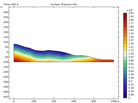
Clear the Color legend checkbox.
10
In the Concentration (tds) toolbar, click  Plot.
Concentration (tds)
1
In the Model Builder window, click Concentration (tds).
2
In the Settings window for 2D Plot Group, click to expand the Title section.
3
From the Title type list, choose Manual.
4
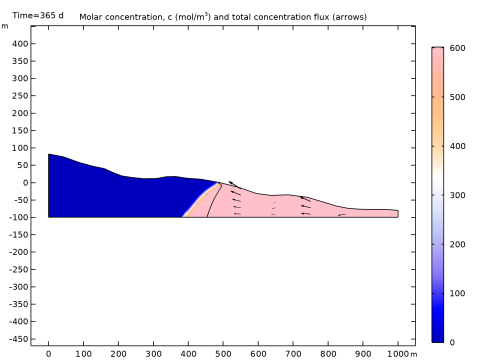
In the Title text area, type Molar concentration, c (mol/m<sup>3</sup>) and total concentration flux (arrows).
5
In the Concentration (tds) toolbar, click  Plot.
6
Click the  Zoom Extents button in the Graphics toolbar.
Precipitation Rate
Lastly, include a plot depicting the precipitation rate. This is an optional element meant to show that the precipitation variability is considered in this model.
1
In the Results toolbar, click  1D Plot Group.
2
In the Settings window for 1D Plot Group, type Precipitation Rate in the Label text field.
Global 1
1
Right-click Precipitation Rate and choose Global.
2
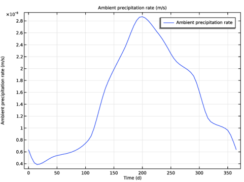
In the Settings window for Global, click Replace Expression in the upper-right corner of the y-Axis Data section. From the menu, choose Component 1 (comp1) > Ambient data > ampr1.P0_amb - Ambient precipitation rate - m/s.
3
Locate the Data section. From the Dataset list, choose Study 2: Dual porosity approach/Solution 2 (sol2).
4
In the Precipitation Rate toolbar, click  Plot.
Study 1: Homogenized approach
Just in case you want to run the homogenized study again, you can deactivate the dual porosity domain conditions in the solver settings for this study as follows:
Step 1: Time Dependent
1
In the Model Builder window, under Study 1: Homogenized approach click Step 1: Time Dependent.
2
In the Settings window for Time Dependent, locate the Physics and Variables Selection section.
3
In the Solve for column of the table, under Component 1 (comp1), clear the checkbox for Domain ODEs and DAEs (dode).
4
Select the Modify model configuration for study step checkbox.
5
In the tree, select Component 1 (comp1) > Darcy’s Law (dl) > Dual Porosity Medium 1.
6
7
In the tree, select Component 1 (comp1) > Transport of Diluted Species in Porous Media (tds) > Heterogeneous Reactions 1.
8