PDF

Reservoir with Horizontal Wells
Introduction
This example models a thin oil reservoir with two horizontal wells, as described in the Seventh SPE Comparative Solution Projects, case 1a (see Ref. 1). This project is about oil recovery by injecting water through a bottom well. The model is used to compute the oil production rate and the water-oil production ratio over time.
Model Definition
The reservoir measures 2700 ft by 2700 ft by 160 ft, and consist of 6 horizontal layers with different initial oil saturations. The thickness of each layer and the initial oil saturation is given in Table 1. The porosity of the reservoir is 0.2 and the horizontal and vertical permeabilities are 300 mD and 30 mD, respectively. The density and the viscosity of both phases are given in Table 2, while the relative permeabilities and capillary pressure (as functions of the water saturation) are given in Table 3.
In the bottom layer water is injected into the reservoir through a horizontal well with a length of 2700 ft. The water pressure at this well is maintained at 3700 psi. The injection well is located at the following coordinates: x = 1350 ft, 0 ft < y < 2700 ft, z = 25 ft.
In the top layer a horizontal well, with a length of 900 ft, produces the fluids at a constant mass flow rate of 5.4181 kg/s, which is the equivalent of 3000 STB of water per day (1 STB, or stock tank barrel, is 0.159 m3). This production well is located at the coordinates x = 1350 ft, 300 ft < y < 1200 ft, z = 150 ft.
The simulation time is 1500 days.
0.96·10-3 Pa·s
0.954·10-3 Pa·s
Results and Discussion
As water is injected through the bottom well, water will start to infiltrate the higher, more oil saturated reservoir layers. This happens especially near the two horizontal wells, as can be seen in Figure 1, where the oil saturation is plotted after the production period of 1500 days: the water table is much higher in between the two wells. This phenomenon is known as coning, and it usually causes a reduction of the oil production rate and an increase in the water-oil production ratio over time.
Figure 1: Oil saturation at the end of the 1500 day production period. Note the elevated water table near the production well.
Figure 2 illustrates this and clearly shows these trends in the present simulation. The results for the oil production and the water-oil ratio agree nicely with the simulation results reported in Ref. 1.
Figure 2: The oil production rate (left y-axis), and the water-oil production ratio (right y-axis) over time.
Notes About the COMSOL Implementation
The prescribed production rate at the production well of 3000 STB/day constitutes a boundary condition for the total mass flow rate, but to solve the model also a boundary condition for the mass flow rate of the oil phase is needed. In the COMSOL model, the oil mass flow rate is determined by requiring that the oil saturation at the production well equals the residual oil saturation (which is equal to 0.2, see Table 3). This condition is implemented using a Well multiphysics edge feature.
Reference
1. L.S. Nghiem, D.A. Collins, and R. Sharma (1991), Seventh SPE Comparative Solution Project: Modelling of Horizontal Wells in Reservoir Simulation, SPE 21221, The 11th SPE Symposium on Reservoir Simulation, Anaheim, CA.
Application Library path: Subsurface_Flow_Module/Fluid_Flow/reservoir_horizontal_wells
Modeling Instructions
From the File menu, choose New.
New
In the New window, click  Model Wizard.
Model Wizard
1
In the Model Wizard window, click  3D.
2
In the Select Physics tree, select Fluid Flow > Porous Media and Subsurface Flow > Multiphase Flow in Porous Media.
3
Click Add.
4
In the Added physics interfaces tree, select Phase Transport in Porous Media (phtr).
5
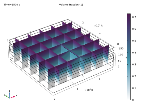
In the Volume fractions (1) table, enter the following settings:
6
Click  Study.
7
In the Select Study tree, select General Studies > Time Dependent.
8
Geometry 1
1
In the Model Builder window, under Component 1 (comp1) click Geometry 1.
2
In the Settings window for Geometry, locate the Units section.
3
From the Length unit list, choose ft.
Block 1 (blk1)
1
In the Geometry toolbar, click  Block.
2
In the Settings window for Block, locate the Size and Shape section.
3
In the Width text field, type 2700.
4
In the Depth text field, type 2700.
5
In the Height text field, type 160.
6
Click to expand the Layers section. Find the Layer position subsection. Clear the Bottom checkbox.
7
Select the Top checkbox.
8
9
Click the  Wireframe Rendering button in the Graphics toolbar.
Line Segment 1 (ls1)
1
In the Geometry toolbar, click  More Primitives and choose Line Segment.
2
In the Settings window for Line Segment, locate the Starting Point section.
3
From the Specify list, choose Coordinates.
4
In the x text field, type 1350.
5
In the z text field, type 25.
6
Locate the Endpoint section. From the Specify list, choose Coordinates.
7
In the x text field, type 1350.
8
In the y text field, type 2700.
9
In the z text field, type 25.
Line Segment 2 (ls2)
1
In the Geometry toolbar, click  More Primitives and choose Line Segment.
2
In the Settings window for Line Segment, locate the Starting Point section.
3
From the Specify list, choose Coordinates.
4
In the x text field, type 1350.
5
In the y text field, type 300.
6
In the z text field, type 150.
7
Locate the Endpoint section. From the Specify list, choose Coordinates.
8
In the x text field, type 1350.
9
In the y text field, type 1200.
10
In the z text field, type 150.
Point 1 (pt1)
1
In the Geometry toolbar, click  More Primitives and choose Point.
2
In the Settings window for Point, locate the Point section.
3
In the x text field, type 1300.
4
In the z text field, type 150.
5
Click  Build Selected, and compare with the image below.
The point is only used later to create an appropriate mesh. In the subsequent step, designate it as a mesh control vertex. This point will then exclusively be part of the mesh sequence and will remain hidden otherwise.
Mesh Control Vertices 1 (mcv1)
1
In the Geometry toolbar, click  Virtual Operations and choose Mesh Control Vertices.
2
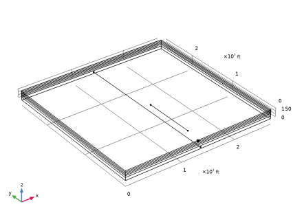
On the object fin, select Point 15 only.
3
In the Geometry toolbar, click  Build All.
Global Definitions
Parameters 1
1
In the Model Builder window, under Global Definitions click Parameters 1.
2
In the Settings window for Parameters, locate the Parameters section.
3
Click  Load from File.
4
Interpolation 1 (int1)
1
In the Home toolbar, click  Functions and choose Global > Interpolation.
2
In the Settings window for Interpolation, locate the Definition section.
3
Click  Load from File.
4
5
In the Function name text field, type krw.
6
Locate the Interpolation and Extrapolation section. From the Interpolation list, choose Piecewise cubic.
Interpolation 2 (int2)
1
In the Home toolbar, click  Functions and choose Global > Interpolation.
2
In the Settings window for Interpolation, locate the Definition section.
3
Click  Load from File.
4
5
In the Function name text field, type krn.
6
Locate the Interpolation and Extrapolation section. From the Interpolation list, choose Piecewise cubic.
Interpolation 3 (int3)
1
In the Home toolbar, click  Functions and choose Global > Interpolation.
2
In the Settings window for Interpolation, locate the Definition section.
3
Click  Load from File.
4
5
In the Function name text field, type pc.
6
Locate the Interpolation and Extrapolation section. From the Interpolation list, choose Piecewise cubic.
Phase Transport in Porous Media (phtr)
1
In the Model Builder window, under Component 1 (comp1) click Phase Transport in Porous Media (phtr).
2
In the Settings window for Phase Transport in Porous Media, locate the Gravity Effects section.
3
Select the Include gravity checkbox.
Fluid 1
1
In the Model Builder window, under Component 1 (comp1) > Phase Transport in Porous Media (phtr) > Porous Medium 1 click Fluid 1.
2
In the Settings window for Fluid, locate the Capillary Pressure section.
3
In the pcsn text field, type pc(sw)[psi].
4
Locate the Phase 1 Properties section. From the ρsw list, choose User defined. In the associated text field, type rhow.
5
From the μsw list, choose User defined. In the associated text field, type muw.
6
7
Locate the Phase 2 Properties section. From the ρsn list, choose User defined. In the associated text field, type rhoo.
8
From the μsn list, choose User defined. In the associated text field, type muo.
9
Initial Values 2
1
In the Physics toolbar, click  Domains and choose Initial Values.
2
3
In the Settings window for Initial Values, locate the Initial Values section.
4
In the s0,sn text field, type 0.711.
Initial Values 3
1
In the Physics toolbar, click  Domains and choose Initial Values.
2
3
In the Settings window for Initial Values, locate the Initial Values section.
4
In the s0,sn text field, type 0.652.
Initial Values 4
1
In the Physics toolbar, click  Domains and choose Initial Values.
2
3
In the Settings window for Initial Values, locate the Initial Values section.
4
In the s0,sn text field, type 0.527.
Initial Values 5
1
In the Physics toolbar, click  Domains and choose Initial Values.
2
3
In the Settings window for Initial Values, locate the Initial Values section.
4
In the s0,sn text field, type 0.351.
Initial Values 6
1
In the Physics toolbar, click  Domains and choose Initial Values.
2
3
In the Settings window for Initial Values, locate the Initial Values section.
4
In the s0,sn text field, type 0.131.
The bottom layer has an initial oil saturation of zero, a condition set by the default Initial Values 1 node.
Darcy’s Law (dl)
Porous Matrix 1
1
In the Model Builder window, under Component 1 (comp1) > Darcy’s Law (dl) > Porous Medium 1 click Porous Matrix 1.
2
In the Settings window for Porous Matrix, locate the Matrix Properties section.
3
From the εp list, choose User defined. In the associated text field, type 0.2.
4
From the κ list, choose User defined. From the list, choose Diagonal.
5
Specify the κ matrix as
Initial Values 1
1
In the Model Builder window, under Component 1 (comp1) > Darcy’s Law (dl) click Initial Values 1.
2
In the Settings window for Initial Values, locate the Initial Values section.
3
In the p text field, type 3700[psi].
Multiphysics
Well 1 (wellmpe1)
1
In the Physics toolbar, click  Multiphysics Couplings and choose Edge > Well.
2
3
In the Settings window for Well, locate the Well section.
4
From the Specify list, choose Pressure.
5
In the p0 text field, type 3700[psi].
Well 2 (wellmpe2)
1
In the Physics toolbar, click  Multiphysics Couplings and choose Edge > Well.
2
3
In the Settings window for Well, locate the Well section.
4
From the Well type list, choose Production.
5
In the M0 text field, type massflow.
6
Locate the Phase 2 section. From the Specify list, choose Volume fraction.
7
In the s0,sn text field, type 0.2.
Mesh 1
Free Triangular 1
1
In the Mesh toolbar, click  More Generators and choose Free Triangular.
2
In the Settings window for Free Triangular, click to expand the Scale Geometry section.
3
In the z-direction scale text field, type 10.
4
Size 1
1
Right-click Free Triangular 1 and choose Size.
2
In the Settings window for Size, locate the Geometric Entity Selection section.
3
From the Geometric entity level list, choose Point.
4
5
Locate the Element Size section. Click the Custom button.
6
Locate the Element Size Parameters section.
7
Select the Maximum element size checkbox. In the associated text field, type 6.
8
Select the Minimum element size checkbox. In the associated text field, type 0.1.
9
Select the Maximum element growth rate checkbox. In the associated text field, type 1.1.
Size
1
In the Model Builder window, under Component 1 (comp1) > Mesh 1 click Size.
2
In the Settings window for Size, locate the Element Size section.
3
From the Predefined list, choose Finer.
Swept 1
1
In the Mesh toolbar, click  Swept.
2
In the Settings window for Swept, click  Build All.
Study 1
Step 1: Time Dependent
1
In the Model Builder window, under Study 1 click Step 1: Time Dependent.
2
In the Settings window for Time Dependent, locate the Study Settings section.
3
From the Time unit list, choose d.
4
In the Output times text field, type range(0,50,1500).
Solution 1 (sol1)
1
In the Study toolbar, click  Show Default Solver.
2
In the Model Builder window, expand the Solution 1 (sol1) node, then click Dependent Variables 1.
3
In the Settings window for Dependent Variables, locate the Scaling section.
4
From the Method list, choose Initial-value based.
5
In the Model Builder window, under Study 1 > Solver Configurations > Solution 1 (sol1) click Time-Dependent Solver 1.
6
In the Settings window for Time-Dependent Solver, click to expand the Time Stepping section.
7
From the Steps taken by solver list, choose Strict.
8
Results
Multislice 1
1
In the Model Builder window, expand the Volume Fraction (phtr) node, then click Multislice 1.
2
In the Settings window for Multislice, locate the Expression section.
3
In the Expression text field, type sn.
4
Locate the Multiplane Data section. Find the x-planes subsection. In the Planes text field, type 5.
5
Find the y-planes subsection. In the Planes text field, type 5.
6
Find the z-planes subsection. In the Planes text field, type 0.
7
In the Volume Fraction (phtr) toolbar, click  Plot.
For a more comprehensive view of the results, employ a scaled view by following these steps.
8
Click the  Show More Options button in the Model Builder toolbar.
9
In the Show More Options dialog, select Results > Views in the tree.
10
11
View 3D 2
In the Model Builder window, under Results right-click Views and choose View 3D.
Camera
1
In the Model Builder window, expand the View 3D 2 node, then click Camera.
2
In the Settings window for Camera, locate the Camera section.
3
From the View scale list, choose Manual.
4
In the z scale text field, type 5.
Volume Fraction (phtr)
1
In the Model Builder window, under Results click Volume Fraction (phtr).
2
In the Settings window for 3D Plot Group, locate the Plot Settings section.
3
From the View list, choose View 3D 2.
4
In the Volume Fraction (phtr) toolbar, click  Plot.
5
Click the  Zoom Extents button in the Graphics toolbar.
1D Plot Group 5
1
In the Results toolbar, click  1D Plot Group.
2
In the Settings window for 1D Plot Group, locate the Data section.
3
From the Time selection list, choose Interpolated.
4
In the Times (d) text field, type range(100,50,1500).
Point Graph 1
1
Right-click 1D Plot Group 5 and choose Point Graph.
2
In the Settings window for Point Graph, locate the Selection section.
3
Click  Paste Selection.
4
In the Paste Selection dialog, type 17 in the Selection text field.
5
6
In the Settings window for Point Graph, locate the y-Axis Data section.
7
In the Expression text field, type wellmpe2.M0_sn/rhoo/STB.
8
In the Unit field, type 1/d.
9
Select the Description checkbox. In the associated text field, type Oil rate (STB/day).
10
Click to expand the Legends section. Select the Show legends checkbox.
11
From the Legends list, choose Manual.
12
Point Graph 2
1
In the Model Builder window, right-click 1D Plot Group 5 and choose Point Graph.
2
In the Settings window for Point Graph, locate the Selection section.
3
Click  Paste Selection.
4
In the Paste Selection dialog, type 17 in the Selection text field.
5
6
In the Settings window for Point Graph, locate the y-Axis Data section.
7
In the Expression text field, type (massflow-wellmpe2.M0_sn)/rhow/(wellmpe2.M0_sn/rhoo).
8
Select the Description checkbox. In the associated text field, type Water-oil ratio.
9
Locate the Legends section. Select the Show legends checkbox.
10
From the Legends list, choose Manual.
11
Oil Rate and Water-Oil Ratio
1
In the Model Builder window, under Results click 1D Plot Group 5.
2
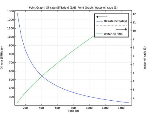
In the Settings window for 1D Plot Group, type Oil Rate and Water-Oil Ratio in the Label text field.
3
Locate the Plot Settings section. Select the Two y-axes checkbox.
4
In the table, select the Plot on secondary y-axis checkbox for Point Graph 2.
5
Select the y-axis label checkbox. In the associated text field, type Oil rate (STB/day).
6
In the Oil Rate and Water-Oil Ratio toolbar, click  Plot. Compare with Figure 2.