PDF

Glacier Flow
Introduction
This example demonstrates the fundamental setup of a glacier flow model. It exemplifies several essential modeling steps in glacier modeling:
The cryosphere is the part of the climate system that contains frozen water and makes up 80% of our fresh water. Using the COMSOL Multiphysics® software, we can simulate classical ice flow to analyze cryosphere dynamics and assess climate change effects such as shrinking glaciers and rising sea levels.
In 1773, André Bordier, a Swiss naturalist, used the term “fluid” to describe the movement of mountain glaciers for the first time. However, it took more than a century for scientists to agree on a unified description for the dynamics of glaciers.
One of the most confusing aspects of glaciers is the observation that ice exhibits both viscous and plastic behavior, depending on the glacier. British physicist John Glen observed and described this intermediate behavior using a nonlinear relationship between stress and strain. Known as shear thinning, this classical behavior applies to many different fluids (for example, ketchup and blood).
The life of any mountain glacier can be schematically described as follows:
Figure 1 shows a sketch of a typical mountain glacier with the accumulation zone where the snow piles up and the ablation zone where the ice melts to water.
Glaciologists divide glaciers in different categories, depending on their thermal structure:
Figure 1: Sketch of a typical mountain glacier.
Most of the alpine glaciers are temperate, but at higher altitudes, also polythermal glaciers can be found. Cold glaciers can typically be found in polar regions like Greenland and Antarctica. Polythermal glaciers are common at high latitudes and high altitudes (like the Scandinavian Mountains, European Alps, Himalaya).
In this example a realistic geometry — a 2D cross section inspired by the Arolla glacier in the Pennine alps in Switzerland — is used to simulate the nonisothermal flow of the ice mass downslope, under its own weight and subject to basal sliding. Two versions of the glacier model are investigated: A cold glacier version and a temperate glacier version.
Model Definition
In this example the geometry is inspired by the Haut glacier d’Arolla in the Swiss Alps, which is 5 kilometers long and up to 200 meters thick with an average slope of 15%. Figure 2 shows a photograph of the Arolla glacier.
Figure 2: Aerial photo of the Arolla glacier in the Pennine Alps in Switzerland.
The model is built in 2D as a cross section through the flow line of the glacier. It is constructed from two datasets, one for the ice surface and one for the bedrock surface. Figure 3 shows the model geometry, colored by the ice thickness.
Figure 3: A 2D cross section of the Arolla glacier is constructed as model geometry. Here it is colored by the ice thickness and the y-axis is stretched compared to the x-axis to have a better view of the vertical differences.
The ice flow is simulated using the Stokes equations describing the so-called creeping flow:
(1)
(2)
where ρ is the density, u is the velocity vector, p is the pressure, g is the acceleration of gravity, and μ is the dynamic viscosity.
Using Glen’s flow law, the viscosity μ can be described as
(3)
where is the shear rate and is classically defined as the norm of the strain rate tensor
(4).
To calculate the flow rate factor A in Equation 3 an Arrhenius law can be used:
(5)
with A0 being the flow rate constant, Q the activation energy, and R the universal gas constant. According to the literature, A0 and Q are a matter of debate. In this case we use,
(6) and
(7).
To calculate the temperature distribution in the model, the energy balance equation is solved:
(8)
where Cp is the heat capacity and k is the thermal conductivity of ice. Both are functions of temperature and are described using the following numerical value equations (see, for example, Ref. 4):
(9) and
(10).
In terms of fluid, the inflow and outflow boundary conditions are the normal constraints, corresponding to the applied pressure of the ice, which is not included in the domain. It simply corresponds to an assigned hydrostatic (or cryostatic) pressure. The upstream boundary weighs on the domain, thus contributing to a streamwise velocity, while the downstream boundary resists to the flow. The surface of the glacier is a free surface.
If the temperature at the ice-bed contact is at the pressure melting temperature Tm — which is the case if the glacier is temperate — the glacier can slide over the base. If the temperature is below Tm a no slip condition would be appropriate. In case of a temperate glacier, a slip length of 50 m is defined at the lower boundary.
In terms of heat transfer, the surface is influenced by the ambient temperature and is subject of convective heat exchange and radiative heat exchange with the environment. For a cold glacier, the boundary in contact with the bedrock is subject to a geothermal heat flux, which could be modeled as a boundary condition. Typical geothermal heat fluxes are of the order of 40–120 mW/m2. In this case a geothermal heat flux of 120 mW/m2 is chosen.
In case the glacier is temperate, the temperature at the bedrock can be assumed to be at pressure melting point temperature, which is
(11)
with Ttp and ptp being the triple point temperature and pressure of water (see Ref. 2). Heat is allowed to leave and enter the domain at the inflow and outflow boundaries.
A mapped mesh is used that is consistent with the aspect ratio of the geometry.
The external weather conditions are an important input data for geophysical simulations. Accessing the ASHRAE 2017 database, you can import the average external temperature and wind velocities at a given time of the year for more than 6000 weather stations all over the world. Here, the data is from the Grand Saint Bernard station in the Swiss Alps, located at about 25 km of the Arolla glacier on the first of February at noon. The ambient temperature is imposed at the glacier surface, and the wind velocities are used to simulate a convective heat flux at the surface.
Results and Discussion
The results are first evaluated after 10 years, when the flow has reached a stationary state. Figure 4 shows the velocity for the “cold glacier” conditions. At the bedrock the velocity is zero and there is hardly any in- and outflow at the upper and lower boundaries. However, there is some uncertainty regarding basal sliding which is not present in this case: Depending on the ice thickness and the geothermal heat flux, even for cold glacier conditions it is possible that a water layer builds up at the bedrock as the heat can only be transported upward very slowly.
Figure 4: Velocity magnitude after 10 years of simulated time for a given heat flux at the bottom (cold glacier model).
The temperature after 10 years of simulation time (Figure 5) shows that the main heat source is the external temperature being in exchange with the glacier surface. Here the highest temperatures occur during summer and the lowest during winter season. The ablation zone of the glacier is colder on average than the accumulation zone. The temperature at the bedrock is higher than in the middle of the glacier due to the geothermal heat flux, however, it is still well below pressure melting temperature.
Figure 5: Temperature distribution after 10 years of simulated time for a given heat flux at the bottom (cold glacier model).
The next figures show the results for the temperate glacier conditions. Here the temperature at the bedrock is set to the pressure melting point temperature (Equation 11), and therefore it can be assumed that the ice can slide over the bedrock. The velocity field, which is displayed in Figure 6, shows this as the velocity is nonzero at the bottom of the glacier. In general the velocities are higher in this case.
Figure 6: Velocity magnitude after 10 years of simulated time for the bottom temperature being at pressure melting point (temperate glacier model).
The temperature distribution after 10 years of simulation time is shown in Figure 7. Again the ablation zone is colder on average than the accumulation zone and the temperature field shows a line structure which is due to a combination of the seasonal heating and cooling from the surface and the influence of the mesh and time step size. With refined mesh the structures still appear on a smaller scale.
Figure 7: Temperature distribution after 10 years of simulated time for the bottom temperature being at pressure melting point temperature (temperate glacier model).
Figure 8 shows the tangential velocity component along the glacier surface for both the cold and the temperate glacier scenario. As already mentioned the velocities are much bigger for the temperate scenario.
Figure 8: Tangential velocity component along the glacier surface after 10 years of simulated time.
References
1. A. Aschwanden and H. Blatter, “Mathematical modeling and numerical simulation of polythermal glaciers,” J. Geophys. Res., vol. 114 (F1), p. F01027, 2008. (10.1029/2008JF001028.)
2. A. Aschwanden, “Thermodynamics of Glaciers,” McCarthy Summer School, 2010. (https://glaciers.gi.alaska.edu/sites/default/files/mccarthy/Notes_thermodyn_Aschwanden.pdf)
3. R. Greve, and H. Blatter, Dynamics of Ice Sheets and Glaciers, Springer, 2009.
4. C. Ritz, “Time dependent boundary conditions for calculation of temperature fields in ice sheets,” The Physical Basis of Ice Sheet Modelling, vol. 170, pp. 207–216, 1987.
Application Library path: Subsurface_Flow_Module/Heat_Transfer/glacier_flow_2d
Modeling Instructions
From the File menu, choose New.
New
In the New window, click  Model Wizard.
Model Wizard
1
In the Model Wizard window, click  2D.
2
In the Select Physics tree, select Fluid Flow > Nonisothermal Flow > Laminar Flow.
3
Click Add.
4
Global Definitions
Parameters 1
1
In the Model Builder window, under Global Definitions click Parameters 1.
Start by setting the parameters defining the material properties of ice and the constants needed to calculate the ice flow. You can either import them from the file "glacier_flow_2d_parameters.txt" from the model’s Application Libraries folder or enter them as follows:
2
In the Settings window for Parameters, locate the Parameters section.
3
Glacier Base
Now import the data to specify the glacier geometry and define the functions to calculate the flow viscosity and the pressure melting temperature.
1
In the Home toolbar, click  Functions and choose Global > Interpolation.
2
In the Settings window for Interpolation, locate the Definition section.
3
From the Data source list, choose File.
4
Click  Browse.
5
6
Click  Import.
7
In the Label text field, type Glacier Base.
8
Locate the Units section. In the Function table, enter the following settings:
9
In the Argument table, enter the following settings:
Glacier Surface
1
In the Home toolbar, click  Functions and choose Global > Interpolation.
2
In the Settings window for Interpolation, locate the Definition section.
3
From the Data source list, choose File.
4
Click  Browse.
5
6
Click  Import.
7
In the Label text field, type Glacier Surface.
8
Locate the Units section. In the Function table, enter the following settings:
9
In the Argument table, enter the following settings:
Now define the flow rate constant A0 and the activation energy Q to calculate the flow rate factor (Equation 5).
A0
1
In the Home toolbar, click  Functions and choose Global > Step.
2
In the Settings window for Step, type A0 in the Label text field.
3
In the Function name text field, type A0.
4
Locate the Parameters section. In the Location text field, type 263.15.
5
In the From text field, type 3.985e-13.
6
In the To text field, type 1.916e3.
7
Click to expand the Smoothing section. Clear the Size of transition zone checkbox.
Q
1
Right-click A0 and choose Duplicate.
2
In the Settings window for Step, type Q in the Label text field.
3
In the Function name text field, type Q.
4
Locate the Parameters section. In the From text field, type 60e3.
5
In the To text field, type 139e3.
Definitions
Define the thermal conductivity, the heat capacity, and the viscosity of ice as variables depending on the temperature T. As T is calculated in Component1, the variables have to be defined locally, that is, in Component1, too.
Variables 1
1
In the Model Builder window, expand the Component 1 (comp1) > Definitions node.
2
Right-click Definitions and choose Variables.
3
In the Settings window for Variables, locate the Variables section.
4
m_ice
1
In the Definitions toolbar, click  Analytic.
2
In the Settings window for Analytic, type m_ice in the Label text field.
3
In the Function name text field, type m_ice.
4
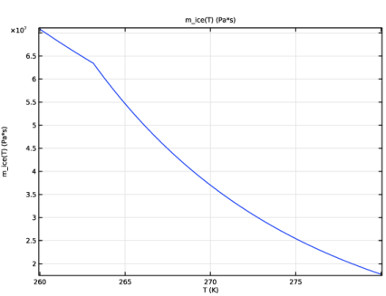
Locate the Definition section. In the Expression text field, type abs(A0(T)*exp(-Q(T)/(R_const*T)))^(-1/3)*0.5  according to Equation 5.
5
In the Arguments text field, type T.
6
Locate the Units section. In the Function text field, type Pa*s.
7
8
Locate the Plot Parameters section. In the table, enter the following settings:
9
Click  Plot  to plot the function and compare with the figure below.
Specify the pressure melting point temperature Tm according to Equation 11.
T_m
1
In the Definitions toolbar, click  Analytic.
2
In the Settings window for Analytic, type T_m in the Label text field.
3
In the Function name text field, type T_m.
4
Locate the Definition section. In the Expression text field, type T_tp-betaCC*(p-p_tp).
5
In the Arguments text field, type p.
6
Locate the Units section. In the Function text field, type K.
7
8
Locate the Plot Parameters section. In the table, enter the following settings:
9
Ambient Properties 1 (ampr1)
Now define the ambient properties. As there is no data for the Arolla glacier directly, select a station where similar weather conditions can be expected.
1
In the Physics toolbar, click  Shared Properties and choose Ambient Properties.
2
In the Settings window for Ambient Properties, locate the Ambient Settings section.
3
From the Ambient data list, choose Meteorological data (ASHRAE 2021).
4
Locate the Location section. Click Set Weather Station.
5
In the Weather Station dialog, select Europe > Switzerland > COL DU GRAND ST BERNARD (067170) in the tree.
6
7
In the Settings window for Ambient Properties, locate the Time section.
8
Find the Date subsection. In the table, enter the following settings:
9
Find the Local time subsection. In the table, enter the following settings:
10
Locate the Ambient Conditions section. From the Temperature list, choose Low.
Geometry 1
Build the geometry using the interpolation functions defined above.
Parametric Curve 1 (pc1)
1
In the Model Builder window, expand the Component 1 (comp1) > Geometry 1 node.
2
Right-click Geometry 1 and choose More Primitives > Parametric Curve.
3
In the Settings window for Parametric Curve, locate the Parameter section.
4
In the Maximum text field, type 5000.
5
Locate the Expressions section. In the x text field, type s.
6
In the y text field, type int1(s).
Parametric Curve 2 (pc2)
1
In the Geometry toolbar, click  More Primitives and choose Parametric Curve.
2
In the Settings window for Parametric Curve, locate the Parameter section.
3
In the Maximum text field, type 5000.
4
Locate the Expressions section. In the x text field, type s.
5
In the y text field, type int2(s).
Line Segment 1 (ls1)
1
In the Geometry toolbar, click  More Primitives and choose Line Segment.
2
On the object pc2, select Point 1 only.
3
In the Settings window for Line Segment, locate the Endpoint section.
4
Click to select the  Activate Selection toggle button for End vertex.
5
On the object pc1, select Point 1 only.
Line Segment 2 (ls2)
1
In the Geometry toolbar, click  More Primitives and choose Line Segment.
2
On the object pc2, select Point 2 only.
3
In the Settings window for Line Segment, locate the Endpoint section.
4
Click to select the  Activate Selection toggle button for End vertex.
5
On the object pc1, select Point 2 only.
Convert to Solid 1 (csol1)
1
In the Geometry toolbar, click  Conversions and choose Convert to Solid.
2
3
Click the  Select All button in the Graphics toolbar.
4
In the Geometry toolbar, click  Build All.
Definitions
Use automatic scaling of the axes to get a better view of the vertical changes within the glacier.
Axis
1
In the Model Builder window, expand the Component 1 (comp1) > Definitions > View 1 node, then click Axis.
2
In the Settings window for Axis, locate the Axis section.
3
From the View scale list, choose Automatic.
4
Click  Update.
5
Click the  Zoom Extents button in the Graphics toolbar.
Materials
Define the material ice in the next step. Introduce it as empty material node, first. As soon as the physics has been defined, the material node menu will show you which properties are needed for the simulation.
Ice
1
In the Model Builder window, under Component 1 (comp1) right-click Materials and choose Blank Material.
2
In the Settings window for Material, type Ice in the Label text field.
Laminar Flow (spf)
Now define the flow properties.
1
In the Model Builder window, under Component 1 (comp1) click Laminar Flow (spf).
2
In the Settings window for Laminar Flow, locate the Physical Model section.
3
Select the Neglect inertial term (Stokes flow) checkbox.
4
Select the Include gravity checkbox.
5
In the pref text field, type ampr1.p_amb.
6
Specify the rref vector as.
This guarantees that the pressure at the ice surface is equal to zero or the ambient pressure, respectively.
Fluid Properties 1
1
In the Model Builder window, under Component 1 (comp1) > Creeping Flow (spf) click Fluid Properties 1.
2
In the Settings window for Fluid Properties, locate the Fluid Properties section.
3
Find the Constitutive relation subsection. From the list, choose Inelastic non-Newtonian. For the Lower shear rate limit enter 1e-15 [1/s].
Wall 2
1
In the Physics toolbar, click  Boundaries and choose Wall.
2
3
In the Settings window for Wall, locate the Boundary Condition section.
4
From the Wall condition list, choose Slip velocity.
5
Select the Use viscous slip checkbox.
6
In the Ls text field, type LSlip. This boundary condition is needed for the temperate glacier model. For the cold glacier flow it has to be disabled.
Open Boundary 1
1
In the Physics toolbar, click  Boundaries and choose Open Boundary.
2
3
In the Settings window for Open Boundary, locate the Boundary Condition section.
4
Clear the Compensate for hydrostatic pressure approximation checkbox.
Open Boundary 2
1
In the Physics toolbar, click  Boundaries and choose Open Boundary.
2
Pressure Point Constraint 1
1
In the Physics toolbar, click  Points and choose Pressure Point Constraint.
2
3
In the Settings window for Pressure Point Constraint, locate the Pressure Constraint section.
4
Clear the Compensate for hydrostatic pressure approximation checkbox.
Heat Transfer in Fluids (ht)
1
In the Model Builder window, under Component 1 (comp1) click Heat Transfer in Fluids (ht).
2
In the Settings window for Heat Transfer in Fluids, locate the Physical Model section.
3
In the dz text field, type 500[m].
Initial Values 1
1
In the Model Builder window, under Component 1 (comp1) > Heat Transfer in Fluids (ht) click Initial Values 1.
2
In the Settings window for Initial Values, locate the Initial Values section.
3
In the T text field, type T_init.
Heat Flux 1
1
In the Physics toolbar, click  Boundaries and choose Heat Flux.
2
3
In the Settings window for Heat Flux, locate the Heat Flux section.
4
In the q0 text field, type q_geo.
Open Boundary 1
1
In the Physics toolbar, click  Boundaries and choose Open Boundary.
2
3
In the Settings window for Open Boundary, locate the Upstream Properties section.
4
From the Tustr list, choose Ambient temperature (ampr1).
Heat Flux 2
1
In the Physics toolbar, click  Boundaries and choose Heat Flux.
2
3
In the Settings window for Heat Flux, locate the Heat Flux section.
4
From the Flux type list, choose Convective heat flux.
5
From the Heat transfer coefficient list, choose External forced convection.
6
In the L text field, type 5000.
7
From the U list, choose Wind speed (ampr1).
8
From the pA list, choose Ambient absolute pressure (ampr1).
9
From the Text list, choose Ambient temperature (ampr1).
Surface-to-Ambient Radiation 1
1
In the Physics toolbar, click  Boundaries and choose Surface-to-Ambient Radiation.
2
3
In the Settings window for Surface-to-Ambient Radiation, locate the Surface-to-Ambient Radiation section.
4
From the ε list, choose User defined. In the associated text field, type 0.97.
5
From the Tamb list, choose Ambient temperature (ampr1).
Temperature 1
1
In the Physics toolbar, click  Boundaries and choose Temperature.
2
3
In the Settings window for Temperature, locate the Temperature section.
4
In the T0 text field, type T_m(p). This boundary condition is needed for the temperate glacier model. For the cold glacier flow it has to be disabled.
Materials
Having defined the physics, now fill in the empty expressions in the Materials node.
Ice (mat1)
1
In the Model Builder window, under Component 1 (comp1) > Materials click Ice (mat1).
2
In the Settings window for Material, locate the Material Contents section.
3
Mesh 1
Mapped 1
In the Mesh toolbar, click  Mapped.
Distribution 1
1
Right-click Mapped 1 and choose Distribution.
2
3
In the Settings window for Distribution, locate the Distribution section.
4
In the Number of elements text field, type 20.
Distribution 2
1
In the Model Builder window, right-click Mapped 1 and choose Distribution.
2
3
In the Settings window for Distribution, locate the Distribution section.
4
In the Number of elements text field, type 100.
5
Click  Build All.
Add Study
Now the flow field and the temperature distribution within the glacier is calculated. Start with a stationary velocity field, first. Therefore, a stationary study step is introduced.
1
In the Home toolbar, click  Add Study to open the Add Study window.
2
Go to the Add Study window.
3
Find the Studies subsection. In the Select Study tree, select General Studies > Stationary.
4
Find the Physics interfaces in study subsection. In the table, clear the Solve checkbox for Heat Transfer in Fluids (ht).
5
Click the Add Study button in the window toolbar.
6
In the Home toolbar, click  Add Study to close the Add Study window.
Study 1
Step 1: Stationary
1
In the Settings window for Stationary, locate the Physics and Variables Selection section.
2
Select the Modify model configuration for study step checkbox.
3
In the tree, select Component 1 (comp1) > Creeping Flow (spf) > Wall 2.
4
Click  Disable  to deactivate the slip boundary condition which is only needed for the temperate glacier simulation.
The next step is to add the time-dependent fully coupled simulation. To catch seasonal variations, force the time-step to be small enough.
Step 2: Time Dependent
1
In the Study toolbar, click  Time Dependent.
2
In the Settings window for Time Dependent, locate the Study Settings section.
3
From the Time unit list, choose a.
4
In the Output times text field, type range(0,0.1,10).
5
Locate the Physics and Variables Selection section. Select the Modify model configuration for study step checkbox.
6
In the tree, select Component 1 (comp1) > Creeping Flow (spf) > Wall 2.
7
Click  Disable.
8
In the tree, select Component 1 (comp1) > Heat Transfer in Fluids (ht) > Temperature 1.
9
Click  Disable.
10
In the Model Builder window, click Study 1.
11
In the Settings window for Study, type Study 1: Cold Glacier in the Label text field.
12
Locate the Study Settings section. Clear the Generate default plots checkbox.
Solution 1 (sol1)
1
In the Study toolbar, click  Show Default Solver.
2
In the Model Builder window, expand the Solution 1 (sol1) node, then click Time-Dependent Solver 1.
3
In the Settings window for Time-Dependent Solver, click to expand the Time Stepping section.
4
From the Steps taken by solver list, choose Strict.
5
In the Study toolbar, click  Compute.
Result Templates
Add plots for the velocity and temperature field from the Result Templates.
1
In the Results toolbar, click  Result Templates to open the Result Templates window.
2
Go to the Result Templates window.
3
In the tree, select Study 1: Cold Glacier/Solution 1 (sol1) > Creeping Flow > Velocity (spf).
4
Click the Add Result Template button in the window toolbar.
5
In the tree, select Study 1: Cold Glacier/Solution 1 (sol1) > Heat Transfer in Fluids > Temperature (ht).
6
Click the Add Result Template button in the window toolbar.
7
In the Results toolbar, click  Result Templates to close the Result Templates window.
Results
Surface
1
In the Model Builder window, expand the Velocity (spf) node, then click Surface.
2
In the Settings window for Surface, locate the Expression section.
3
In the Unit field, type m/yr.
4
In the Velocity (spf) toolbar, click  Plot.
Line Average 1
As an additional plot, the outward mass flow rate, averaged over the glacier surface and the lower end of the glacier are plotted here as follows.
1
In the Results toolbar, click  More Derived Values and choose Average > Line Average.
2
3
In the Settings window for Line Average, click Replace Expression in the upper-right corner of the Expressions section. From the menu, choose Component 1 (comp1) > Creeping Flow > Auxiliary variables > spf.open1.massFlowRate - Outward mass flow rate across feature selection - kg/s.
4
Click  Evaluate.
Table 1
1
Go to the Table 1 window.
2
Click the Table Graph button in the window toolbar.
Results
Outward Mass Flow Rate
1
In the Model Builder window, under Results click 1D Plot Group 3.
2
In the Settings window for 1D Plot Group, type Outward Mass Flow Rate in the Label text field.
Temperate Glacier
Add Study
Now add a second study and modify the boundary conditions to match the conditions for a temperate glacier. Start again with a stationary study. This time, as flow and heat transfer are strongly coupled due to the lower boundary condition, a stationary solution of both velocity and temperature fields is calculated.
1
In the Home toolbar, click  Add Study to open the Add Study window.
2
Go to the Add Study window.
3
Find the Studies subsection. In the Select Study tree, select General Studies > Stationary.
4
5
In the Home toolbar, click  Add Study to close the Add Study window.
Study 2
Step 2: Time Dependent
In the Study toolbar, click  Time Dependent.
Step 1: Stationary
1
In the Settings window for Stationary, locate the Physics and Variables Selection section.
2
Select the Modify model configuration for study step checkbox.
3
In the tree, select Component 1 (comp1) > Heat Transfer in Fluids (ht) > Heat Flux 1.
4
Right-click and choose Disable   to deactivate the heat flux boundary condition that is only needed for the cold glacier simulation, not the temperate glacier simulation.
Step 2: Time Dependent
1
In the Model Builder window, click Step 2: Time Dependent.
2
In the Settings window for Time Dependent, locate the Study Settings section.
3
From the Time unit list, choose a.
4
In the Output times text field, type range(0,0.1,10).
5
Locate the Physics and Variables Selection section. Select the Modify model configuration for study step checkbox.
6
In the tree, select Component 1 (comp1) > Heat Transfer in Fluids (ht) > Heat Flux 1.
7
8
In the Model Builder window, click Study 2.
9
In the Settings window for Study, type Study 2: Temperate Glacier in the Label text field.
10
Locate the Study Settings section. Clear the Generate default plots checkbox.
Solution 3 (sol3)
1
In the Study toolbar, click  Show Default Solver.
2
In the Model Builder window, expand the Solution 3 (sol3) node, then click Time-Dependent Solver 1.
3
In the Settings window for Time-Dependent Solver, locate the Time Stepping section.
4
From the Steps taken by solver list, choose Strict.
5
Select the Initial step checkbox. In the associated text field, type 1[s].
6
In the Study toolbar, click  Compute.
Results
The same plots as for the Cold Glacier should be produced. Therefore, just duplicate them and update which solution they should take. First, compute the Outward Mass Flow Rate
Line Average 2
1
In the Model Builder window, under Results > Derived Values right-click Line Average 1 and choose Duplicate.
2
In the Settings window for Line Average, locate the Data section.
3
From the Dataset list, choose Study 2: Temperate Glacier/Solution 3 (sol3).
4
Clicknext to  Evaluate, then choose New Table.
Outward Mass Flow Rate, Temperature (ht), Velocity (spf)
Group the existing plots into a group and then duplicate them to update them with the solution for the temperate glacier.
1
In the Model Builder window, under Results, Ctrl-click to select Velocity (spf), Temperature (ht), and Outward Mass Flow Rate.
2
Cold Glacier
In the Settings window for Group, type Cold Glacier in the Label text field.
Temperate Glacier
1
Right-click Cold Glacier and choose Duplicate.
2
In the Settings window for Group, type Temperate Glacier in the Label text field.
Velocity (spf) 1
1
In the Model Builder window, expand the Temperate Glacier node, then click Velocity (spf) 1.
2
In the Settings window for 2D Plot Group, locate the Data section.
3
From the Dataset list, choose Study 2: Temperate Glacier/Solution 3 (sol3).
4
In the Velocity (spf) 1 toolbar, click  Plot.
Temperature (ht) 1
1
In the Model Builder window, click Temperature (ht) 1.
2
In the Settings window for 2D Plot Group, locate the Data section.
3
From the Dataset list, choose Study 2: Temperate Glacier/Solution 3 (sol3).
4
In the Temperature (ht) 1 toolbar, click  Plot.
Outward Mass Flow Rate 1
1
In the Model Builder window, expand the Outward Mass Flow Rate 1 node, then click Table Graph 1.
2
In the Settings window for Table Graph, locate the Data section.
3
From the Table list, choose Table 2.
4
In the Label text field, type Outward Mass Flow Rate 1.
5
In the Outward Mass Flow Rate 1 toolbar, click  Plot.
Plot the ice thickness as in Figure 3 as follows.
Ice Thickness
1
In the Results toolbar, click  2D Plot Group.
2
In the Settings window for 2D Plot Group, type Ice Thickness in the Label text field.
Surface 1
1
Right-click Ice Thickness and choose Surface.
2
In the Settings window for Surface, locate the Expression section.
3
In the Expression text field, type abs(int1(x)-int2(x)).
4
Locate the Coloring and Style section. From the Color table list, choose JupiterAuroraBorealis.
5
In the Ice Thickness toolbar, click  Plot.
1D Plot Group 8
To compare the tangential velocities along the glacier surface as displayed in Figure 8, follow the steps below.
In the Results toolbar, click  1D Plot Group.
Line Graph 1
1
Right-click 1D Plot Group 8 and choose Line Graph.
2
3
In the Settings window for Line Graph, locate the y-Axis Data section.
4
In the Expression text field, type u*tx+v*ty.
5
In the Unit field, type m/yr.
6
Click to expand the Legends section. Select the Show legends checkbox.
7
From the Legends list, choose Manual.
8
1D Plot Group 8
1
In the Model Builder window, click 1D Plot Group 8.
2
In the Settings window for 1D Plot Group, locate the Data section.
3
From the Time selection list, choose Last.
Line Graph 2
1
Right-click 1D Plot Group 8 and choose Line Graph.
2
In the Settings window for Line Graph, locate the Data section.
3
From the Dataset list, choose Study 2: Temperate Glacier/Solution 3 (sol3).
4
From the Time selection list, choose Last.
5
6
Locate the y-Axis Data section. In the Expression text field, type u*tx+v*ty.
7
In the Unit field, type m/yr.
8
Locate the Legends section. Select the Show legends checkbox.
9
From the Legends list, choose Manual.
10
Tangential Velocity along Glacier Surface
1
In the Model Builder window, under Results click 1D Plot Group 8.
2
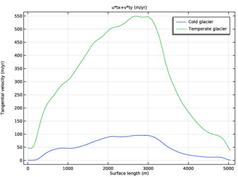
In the Settings window for 1D Plot Group, type Tangential Velocity along Glacier Surface in the Label text field.
3
In the Tangential Velocity along Glacier Surface toolbar, click  Plot.
4
Locate the Plot Settings section.
5
Select the x-axis label checkbox. In the associated text field, type Surface length (m).
6
Select the y-axis label checkbox. In the associated text field, type Tangential velocity (m/yr).
Line Graph 2
1
In the Model Builder window, click Line Graph 2.
2
In the Settings window for Line Graph, click to expand the Title section.
3
From the Title type list, choose None.