
|
|
|
|
1
|
|
2
|
In the Select Physics tree, select Fluid Flow > Porous Media and Subsurface Flow > Darcy’s Law (dl).
|
|
3
|
Click Add.
|
|
4
|
In the Select Physics tree, select Heat Transfer > Porous Media > Heat Transfer in Porous Media (ht).
|
|
5
|
Click Add.
|
|
6
|
Click
|
|
7
|
|
8
|
Click
|
|
1
|
|
2
|
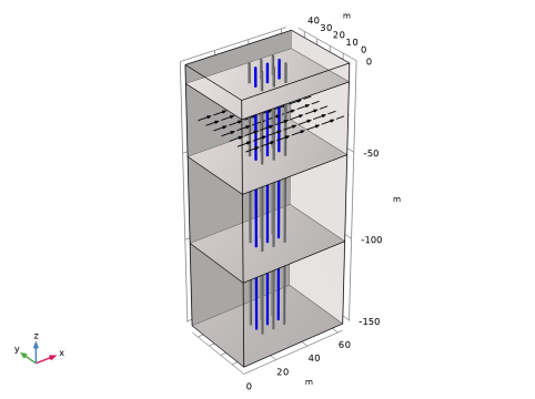
Browse to the model’s Application Libraries folder and double-click the file borehole_heat_exchanger_geom_sequence.mph.
|
|
3
|
|
1
|
|
2
|
|
1
|
Go to the Add Material window.
|
|
2
|
|
3
|
Click the Add to Component button in the window toolbar.
|
|
4
|
|
1
|
In the Model Builder window, under Component 1 (comp1) right-click Materials and choose More Materials > Porous Material.
|
|
2
|
In the Settings window for Porous Material, type Porous Material: Holocene Sediments in the Label text field.
|
|
3
|
|
4
|
|
1
|
|
2
|
|
3
|
|
1
|
|
2
|
|
3
|
|
4
|
Locate the Material Contents section. In the table, enter the following settings:
|
|
1
|
In the Model Builder window, under Component 1 (comp1) right-click Materials and choose More Materials > Porous Material.
|
|
2
|
In the Settings window for Porous Material, type Porous Material: Pleistocene Sands in the Label text field.
|
|
3
|
|
4
|
|
1
|
|
2
|
|
3
|
|
1
|
|
2
|
|
3
|
|
4
|
Locate the Material Contents section. In the table, enter the following settings:
|
|
1
|
In the Model Builder window, under Component 1 (comp1) right-click Materials and choose More Materials > Porous Material.
|
|
2
|
|
3
|
|
4
|
|
5
|
|
1
|
|
2
|
|
3
|
|
1
|
|
2
|
|
3
|
|
4
|
Locate the Material Contents section. In the table, enter the following settings:
|
|
1
|
In the Model Builder window, under Component 1 (comp1) right-click Materials and choose More Materials > Porous Material.
|
|
2
|
In the Settings window for Porous Material, type Porous Material: Tertiary Sands in the Label text field.
|
|
3
|
|
4
|
|
1
|
|
2
|
|
3
|
|
1
|
|
2
|
|
3
|
|
4
|
Locate the Material Contents section. In the table, enter the following settings:
|
|
1
|
In the Model Builder window, under Component 1 (comp1) > Materials click Porous Material: Holocene Sediments (pmat1).
|
|
2
|
|
1
|
|
2
|
|
1
|
|
2
|
|
3
|
|
4
|
|
5
|
|
6
|
Click OK.
|
|
1
|
|
2
|
|
3
|
Click
|
|
5
|
|
1
|
|
2
|
|
3
|
Click
|
|
5
|
|
1
|
|
2
|
|
3
|
Click the Hydraulic head button.
|
|
1
|
|
2
|
|
3
|
|
1
|
|
3
|
|
4
|
|
1
|
|
2
|
|
3
|
|
4
|
|
5
|
|
7
|
Locate the Plot Parameters section. In the table, enter the following settings:
|
|
8
|
Click
|
|
1
|
In the Model Builder window, under Component 1 (comp1) > Heat Transfer in Porous Media (ht) > Porous Medium 1 click Porous Matrix 1.
|
|
2
|
|
3
|
|
1
|
In the Model Builder window, under Component 1 (comp1) > Heat Transfer in Porous Media (ht) click Initial Values 1.
|
|
2
|
|
3
|
|
1
|
|
1
|
|
2
|
|
3
|
|
1
|
|
2
|
|
3
|
|
1
|
|
3
|
|
4
|
|
1
|
|
3
|
|
4
|
|
1
|
|
3
|
|
4
|
|
1
|
|
2
|
|
3
|
|
4
|
|
5
|
|
1
|
|
1
|
|
2
|
|
3
|
|
1
|
|
2
|
|
3
|
|
5
|
|
6
|
Locate the Element Size Parameters section.
|
|
7
|
|
8
|
Click
|
|
1
|
|
2
|
|
3
|
Click
|
|
5
|
|
1
|
|
2
|
|
3
|
Click
|
|
5
|
|
6
|
Click
|
|
1
|
|
2
|
|
3
|
Clear the Generate default plots checkbox.
|
|
1
|
|
2
|
|
3
|
|
4
|
|
1
|
|
2
|
|
3
|
|
4
|
From the Steps taken by solver list, choose Strict to ensure that the changes of the ambient temperature are represented properly.
|
|
1
|
|
2
|
Go to the Result Templates window.
|
|
3
|
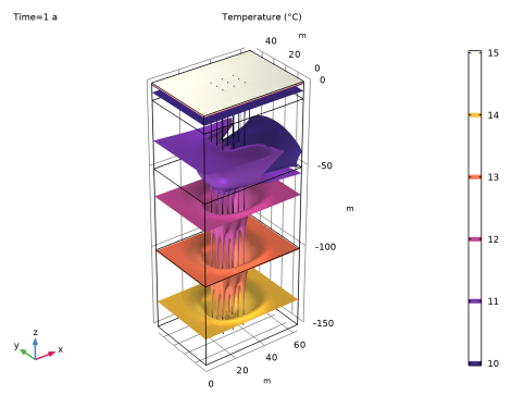
In the tree, select Study 1/Solution 1 (sol1) > Heat Transfer in Porous Media > Temperature, Multislice (ht) and Study 1/Solution 1 (sol1) > Heat Transfer in Porous Media > Isothermal Contours (ht).
|
|
4
|
Click the Add Result Template button in the window toolbar.
|
|
5
|
|
1
|
|
2
|
|
3
|
|
4
|
|
5
|
|
6
|
|
7
|
|
8
|
|
9
|
|
10
|
|
1
|
|
2
|
|
3
|
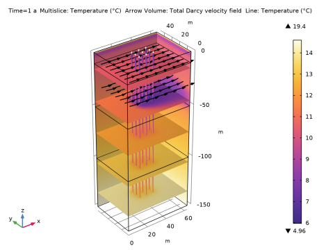
Select the Show maximum and minimum values checkbox.
|
|
1
|
|
2
|
In the Settings window for Arrow Volume, click Replace Expression in the upper-right corner of the Expression section. From the menu, choose Component 1 (comp1) > Darcy’s Law > Velocity and pressure > dl.u,dl.v,dl.w - Total Darcy velocity field.
|
|
3
|
|
1
|
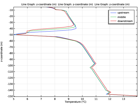
Right-click Temperature, Multislice (ht) and choose Line to add the temperatures around the boreholes to the plot.
|
|
2
|
|
3
|
|
4
|
|
5
|
|
6
|
|
7
|
|
1
|
|
2
|
|
3
|
|
4
|
|
5
|
|
6
|
|
1
|
|
2
|
|
3
|
|
4
|
|
5
|
|
6
|
|
7
|
|
1
|
|
2
|
|
3
|
|
4
|
|
5
|
|
1
|
|
2
|
|
3
|
|
4
|
|
5
|
|
6
|
|
7
|
|
8
|
|
9
|
|
10
|
|
11
|
|
1
|
|
2
|
|
3
|
Click
|
|
4
|
Select Edges 40–43 only. You could again use the Go to XY View and the Select Box buttons from the graphics toolbar to select the edges corresponding to the middle borehole.
|
|
5
|
Locate the Legends section. In the table, enter the following settings:
|
|
1
|
|
2
|
|
3
|
Click
|
|
4
|
|
5
|
Locate the Legends section. In the table, enter the following settings:
|
|
6
|
|
7
|
|
1
|
|
2
|
|
3
|
Select the Manual axis limits checkbox.
|
|
4
|
|
5
|
|
6
|
|
7
|