|









|
1
|
|
2
|
In the Select Physics tree, select Heat Transfer > Porous Media > Heat Transfer in Porous Media (ht).
|
|
3
|
Click Add.
|
|
4
|
Click
 Study. Study. |
|
5
|
|
6
|
Click
 Done. Done. |
|
1
|
|
2
|
Browse to the model’s Application Libraries folder and double-click the file artificial_ground_freezing_geom_sequence.mph.
|
|
3
|
|
4
|
|
1
|
|
2
|
|
3
|
Click
 Load from File. Load from File. |
|
4
|
Browse to the model’s Application Libraries folder and double-click the file artificial_ground_freezing_parameters.txt.
|
|
1
|
|
2
|
|
3
|
|
4
|
|
5
|
|
6
|
|
8
|
Locate the Plot Parameters section. In the table, enter the following settings:
|
|
9
|
|
1
|
|
2
|
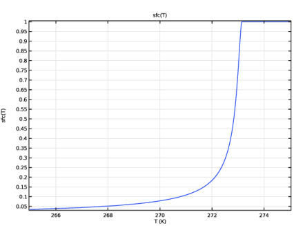
In the Settings window for Analytic, type Soil Freezing Characteristic Curve in the Label text field.
|
|
3
|
|
4
|
Locate the Definition section. In the Expression text field, type if(T<273.15[K], (1+abs(eta*hcs(T))^(1/(1-n)))^(-n), 1).
|
|
5
|
|
6
|
Locate the Units section. In the table, enter the following settings:
|
|
7
|
Click to expand the Local Parameters section. In the table, enter the following settings:
|
|
8
|
Locate the Plot Parameters section. In the table, enter the following settings:
|
|
9
|
Click
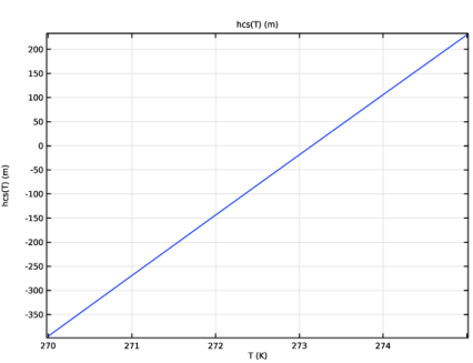
 Plot and compare with the plot below. Plot and compare with the plot below. |
|
1
|
|
2
|
|
1
|
In the Model Builder window, under Component 1 (comp1) right-click Materials and choose Blank Material.
|
|
2
|
|
1
|
|
2
|
|
1
|
|
1
|
|
2
|
|
3
|
|
4
|
|
5
|
|
6
|
|
1
|
In the Model Builder window, under Component 1 (comp1) > Heat Transfer in Porous Media (ht) > Porous Medium 1 click Porous Matrix 1.
|
|
2
|
|
3
|
|
1
|
In the Model Builder window, under Component 1 (comp1) > Heat Transfer in Porous Media (ht) click Initial Values 1.
|
|
2
|
|
3
|
|
1
|
|
3
|
|
4
|
|
1
|
|
2
|
|
3
|
|
4
|
|
5
|
|
1
|
|
2
|
|
3
|
|
4
|
|
5
|
|
6
|
|
1
|
|
2
|
|
3
|
|
4
|
|
5
|
|
6
|
|
1
|
|
2
|
Go to the Add Physics window.
|
|
3
|
|
4
|
Click the Add to Component 1 button in the window toolbar.
|
|
5
|
|
1
|
|
1
|
|
1
|
|
2
|
|
3
|
|
1
|
|
2
|
|
3
|
Select the Include gravity checkbox.
|
|
4
|
|
1
|
In the Model Builder window, under Component 1 (comp1) > Darcy’s Law (dl) > Porous Medium 1 click Porous Matrix 1.
|
|
2
|
|
3
|
|
1
|
|
2
|
|
3
|
Click the Hydraulic head button.
|
|
1
|
|
3
|
|
4
|
|
1
|
|
3
|
|
4
|
|
1
|
|
1
|
|
2
|
Go to the Add Multiphysics window.
|
|
3
|
In the tree, select No Predefined Multiphysics Available for the Selected Physics Interfaces.
|
|
4
|
Find the Select the physics interfaces you want to couple subsection. In the table, clear the Couple checkbox for Darcy’s Law (dl).
|
|
5
|
|
6
|
Click the Add to Component button in the window toolbar.
|
|
7
|
|
1
|
|
2
|
|
3
|
|
1
|
In the Model Builder window, under Component 1 (comp1) > Heat Transfer in Porous Media (ht) > Porous Medium 1 click Fluid 1.
|
|
2
|
|
3
|
|
1
|
|
2
|
|
3
|
|
4
|
|
5
|
|
6
|
Locate the Local Parameters section. In the table, enter the following settings:
|
|
7
|
|
1
|
In the Model Builder window, expand the Component 1 (comp1) > Materials > Porous Material 1 (pmat1) node, then click Porous Material 1 (pmat1).
|
|
2
|
|
3
|
Click
 Add Required Phase Nodes. Add Required Phase Nodes. |
|
1
|
|
2
|
|
3
|
|
1
|
|
2
|
|
3
|
|
4
|
Locate the Material Contents section. In the table, enter the following settings:
|
|
1
|
|
2
|
|
1
|
|
2
|
|
1
|
|
2
|
|
1
|
|
1
|
|
2
|
Click the
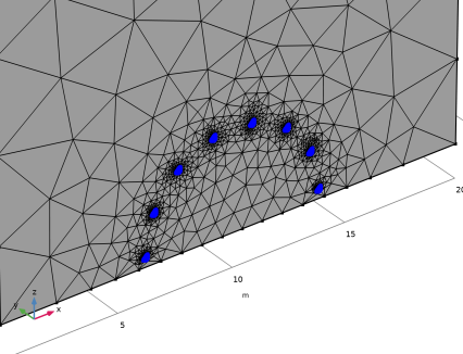
 Select Box button in the Graphics toolbar. Draw a box around all pipe edges on the surface that is about to be meshed. This corresponds to the following. Select Box button in the Graphics toolbar. Draw a box around all pipe edges on the surface that is about to be meshed. This corresponds to the following. |
|
4
|
|
1
|
|
2
|
|
3
|
|
4
|
Click the Custom button.
|
|
5
|
|
6
|
|
1
|
|
2
|
|
3
|
Click the Custom button.
|
|
4
|
Locate the Element Size Parameters section.
|
|
5
|
|
6
|
Click
 Build All. Build All. |
|
1
|
|
2
|
|
3
|
Clear the Generate default plots checkbox.
|
|
1
|
|
2
|
|
3
|
|
4
|
|
1
|
|
2
|
|
3
|
Select the Modify model configuration for study step checkbox.
|
|
4
|
|
5
|
Click
 Disable. Disable. |
|
6
|
|
1
|
|
2
|
|
3
|
|
4
|
|
5
|
|
1
|
|
2
|
|
3
|
|
1
|
|
2
|
|
3
|
|
4
|
|
1
|
|
2
|
In the Settings window for Streamline, click Replace Expression in the upper-right corner of the Expression section. From the menu, choose Component 1 (comp1) > Darcy’s Law > Velocity and pressure > dl.u,...,dl.w - Total Darcy velocity field (spatial frame).
|
|
3
|
|
4
|
|
5
|
|
6
|
Locate the Coloring and Style section. Find the Point style subsection. From the Type list, choose Arrow.
|
|
7
|
|
1
|
|
2
|
In the Settings window for Surface, click Replace Expression in the upper-right corner of the Expression section. From the menu, choose Component 1 (comp1) > Solid Mechanics > Stress > solid.misesGp - von Mises stress - N/m².
|
|
3
|
|
1
|
|
2
|
|
3
|
Select the Plot checkbox.
|
|
4
|
|
1
|
In the Model Builder window, expand the Study 1 > Solver Configurations > Solution 1 (sol1) node, then click Time-Dependent Solver 1.
|
|
2
|
|
3
|
|
4
|
Select the Initial step checkbox. In the associated text field, type 1[h] to capture the initial temperature drop in and around the pipes.
|
|
5
|
|
1
|
|
2
|
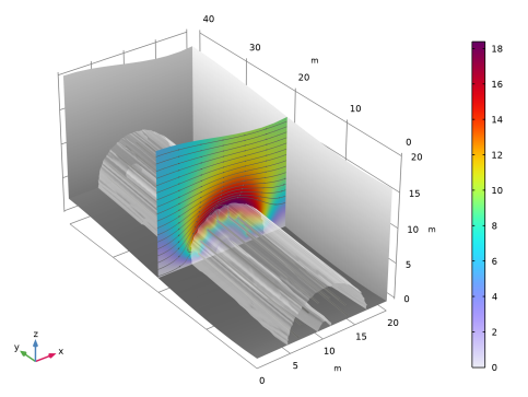
In the Settings window for 3D Plot Group, type Freezing Front and Deformation in the Label text field.
|
|
1
|
|
2
|
|
3
|
|
4
|
|
5
|
|
6
|
|
7
|
|
8
|
Clear the Color legend checkbox.
|
|
1
|
|
2
|
|
3
|
|
4
|
|
5
|
Click Replace Expression in the upper-right corner of the Expression section. From the menu, choose Component 1 (comp1) > Solid Mechanics > Displacement > solid.disp - Displacement magnitude - m.
|
|
6
|
|
7
|
|
1
|
|
2
|
|
3
|
|
4
|
|
5
|
Click Replace Expression in the upper-right corner of the Expression section. From the menu, choose Component 1 (comp1) > Darcy’s Law > Velocity and pressure > dl.u,...,dl.w - Total Darcy velocity field (spatial frame).
|
|
6
|
|
7
|
|
8
|
|
9
|
|
10
|
Locate the Coloring and Style section. Find the Point style subsection. From the Type list, choose Arrow.
|
|
11
|
|
12
|
On Windows, click the colored bar underneath, or — if you are running the cross-platform desktop — the Color button and select a dark gray tone.
|
|
1
|
|
2
|
|
3
|
|
4
|
|
5
|
|
6
|
|
7
|
Click Define custom colors.
|
|
9
|
Click Add to custom colors.
|
|
10
|
|
1
|
|
1
|
|
2
|
|
3
|
|
1
|
|
2
|
|
3
|
|
4
|
|
1
|
|
2
|
|
3
|
Clear the Plot dataset edges checkbox.
|
|
4
|
|
5
|
|
6
|
|
7
|
|
1
|
|
2
|
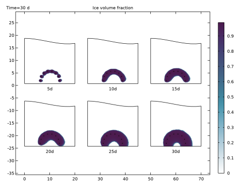
In the Settings window for 2D Plot Group, type Ice Saturation at Different Times in the Label text field.
|
|
3
|
|
4
|
|
5
|
|
6
|
|
1
|
|
2
|
|
3
|
|
4
|
|
1
|
|
2
|
|
3
|
|
4
|
|
5
|
|
1
|
|
2
|
|
3
|
|
5
|
|
6
|
|
7
|
|
8
|
|
1
|
|
1
|
|
2
|
|
3
|
|
4
|
|
5
|
|
6
|
|
7
|
|
8
|
Select the Additional parallel lines checkbox.
|
|
9
|
|
10
|
Click
 PlotThe lines are at the bottom surface in upstream direction. PlotThe lines are at the bottom surface in upstream direction. |
|
11
|
Click to expand the Advanced section.
|
|
1
|
|
2
|
|
3
|
|
4
|
|
5
|
|
6
|
|
7
|
|
9
|
Click
 Evaluate. Evaluate. |
|
1
|
Go to the Table 1 window.
|
|
2
|
Click the Table Graph button in the window toolbar.
|
|
1
|
|
2
|
|
3
|
In the Columns list, choose Ice thickness based on ice saturation (m), Ice thickness based on ice saturation (m), Distance=10, Ice thickness based on ice saturation (m), Distance=20, and Ice thickness based on ice saturation (m), Distance=30.
|
|
4
|
|
5
|
|
6
|
|
1
|
|
2
|
|
3
|
In the Columns list, choose Ice thickness based on temperature isotherm) (m), Ice thickness based on temperature isotherm) (m), Distance=10, Ice thickness based on temperature isotherm) (m), Distance=20, and Ice thickness based on temperature isotherm) (m), Distance=30.
|
|
4
|
|
5
|
Locate the Coloring and Style section. Find the Line style subsection. From the Line list, choose Dotted.
|
|
6
|
|
1
|
|
2
|
|
3
|
|
4
|
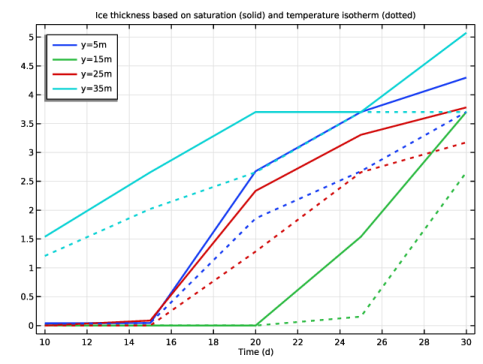
In the Title text area, type Ice thickness based on saturation (solid) and temperature isotherm (dotted).
|
|
5
|
|
6
|
 .
.