|
|
|

|
•
|
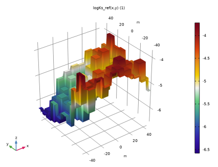
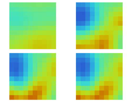
A text file with reference synthetically generated field data, containing the log10 values of the regularized hydraulic-conductivity parameter field that is used to generate fictitious hydraulic-head measurements. This allows you to evaluate the optimization solver’s performance and accuracy, and to test and calibrate the inverse model. For example, you can try out different penalty terms in the objective function and investigate the solution’s dependence on the number of observations used.
|
|
1
|
|
2
|
In the Select Physics tree, select Fluid Flow > Porous Media and Subsurface Flow > Darcy’s Law (dl).
|
|
3
|
Click Add.
|
|
4
|
Click
|
|
5
|
|
6
|
Click
|
|
1
|
|
2
|
|
3
|
|
4
|
|
5
|
|
1
|
|
2
|
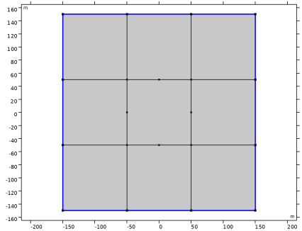
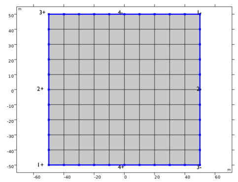
Select the object sq1 only.
|
|
3
|
|
4
|
|
5
|
|
6
|
|
7
|
|
1
|
|
2
|
|
3
|
|
4
|
|
5
|
|
6
|
|
1
|
|
2
|
|
1
|
|
2
|
|
3
|
|
4
|
Click
|
|
5
|
Browse to the model’s Application Libraries folder and double-click the file aquifer_characterization_logKs_ref.txt.
|
|
6
|
|
7
|
Click
|
|
8
|
|
9
|
Locate the Definition section. Find the Functions subsection. In the table, enter the following settings:
|
|
10
|
Locate the Interpolation and Extrapolation section. From the Interpolation list, choose Nearest neighbor.
|
|
11
|
|
12
|
In the Argument table, enter the following settings:
|
|
13
|
|
1
|
|
1
|
In the Model Builder window, under Component 1 (comp1) right-click Definitions and choose Variables.
|
|
2
|
|
3
|
Locate the Variables section. In the table, enter the following settings:
|
|
1
|
|
2
|
Go to the Add Material window.
|
|
3
|
|
4
|
Click the Add to Component button in the window toolbar.
|
|
5
|
|
1
|
|
2
|
|
3
|
In the K text field, type 10^logKs0. This is the conductivity that is applied to the Infinite Element Domain. The center domain is defined as follows:
|
|
1
|
|
1
|
|
2
|
|
3
|
|
4
|
|
1
|
|
1
|
|
3
|
|
4
|
|
1
|
|
2
|
|
3
|
From the list, choose User-controlled mesh.
|
|
1
|
|
2
|
|
3
|
|
5
|
|
6
|
Locate the Element Size Parameters section.
|
|
7
|
|
1
|
|
2
|
|
3
|
|
5
|
|
6
|
Locate the Element Size Parameters section.
|
|
7
|
|
8
|
|
1
|
|
2
|
|
3
|
Locate the Study Settings section. Clear the Generate default plots checkbox because you add the relevant plots from the Result Templates after the computation.
|
|
4
|
|
1
|
|
2
|
Go to the Result Templates window.
|
|
3
|
|
4
|
Click the Add Result Template button in the window toolbar.
|
|
5
|
|
6
|
Click the Add Result Template button in the window toolbar.
|
|
7
|
|
1
|
|
1
|
|
2
|
|
1
|
|
2
|
Go to the Add Physics window.
|
|
3
|
|
4
|
Click the Add to Component 2 button in the window toolbar.
|
|
5
|
|
1
|
|
2
|
Go to the Add Study window.
|
|
3
|
|
4
|
Click the Add Study button in the window toolbar.
|
|
5
|
|
1
|
|
2
|
|
3
|
|
4
|
|
1
|
|
2
|
|
3
|
|
1
|
|
2
|
|
3
|
|
4
|
|
1
|
|
2
|
|
3
|
|
5
|
Locate the Variables section. In the table, enter the following settings:
|
|
1
|
|
2
|
|
3
|
Locate the Variables section. In the table, enter the following settings:
|
|
1
|
|
2
|
In the Settings window for Domain Probe, type Area-weighted mean squared error in the Label text field.
|
|
3
|
|
4
|
|
1
|
|
2
|
|
3
|
|
4
|
|
5
|
Locate the Units section. In the table, enter the following settings:
|
|
6
|
|
1
|
|
2
|
|
3
|
|
4
|
|
5
|
Locate the Discretization section. From the Shape function type list, choose Discontinuous Lagrange.
|
|
6
|
|
1
|
|
2
|
|
3
|
|
4
|
Click
|
|
5
|
Locate the Data Column Settings section. In the table, enter the following settings:
|
|
6
|
|
7
|
|
8
|
|
1
|
|
2
|
|
3
|
In the Source term quantity table, enter the following settings:
|
|
4
|
|
1
|
In the Model Builder window, under Component 2 (comp2) > Domain ODEs and DAEs (dode) click Distributed ODE 1.
|
|
2
|
|
3
|
|
1
|
|
2
|
|
3
|
|
4
|
|
5
|
Click
|
|
1
|
|
2
|
|
3
|
Locate the Variables section. In the table, enter the following settings:
|
|
1
|
|
2
|
|
3
|
|
4
|
|
5
|
Locate the Experimental Data section. In the Filename text field, type aquifer_characterization_H1.csv.
|
|
6
|
Click
|
|
7
|
Locate the Data Column Settings section. In the table, enter the following settings:
|
|
8
|
|
10
|
|
11
|
|
12
|
|
13
|
|
14
|
|
1
|
|
2
|
|
3
|
Locate the Physics and Variables Selection section. Select the Modify model configuration for study step checkbox.
|
|
4
|
|
5
|
Click
|
|
6
|
|
7
|
|
8
|
Clear the Generate default plots checkbox.
|
|
9
|
|
1
|
|
2
|
|
3
|
|
1
|
|
2
|
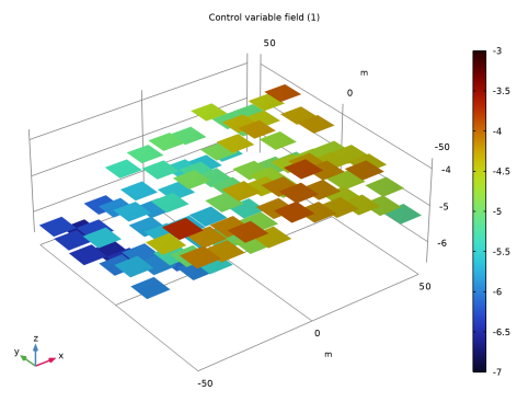
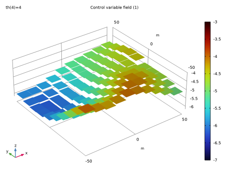
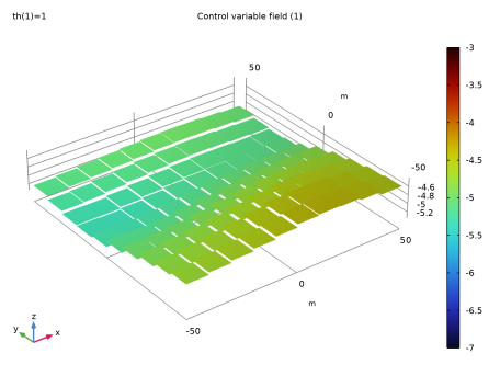
In the Settings window for Surface, click Replace Expression in the upper-right corner of the Expression section. From the menu, choose Component 2 (comp2) > Definitions > Control Variable Field 1 > logKs - Control variable field - 1.
|
|
3
|
|
4
|
|
5
|
|
6
|
|
7
|
|
8
|
|
1
|
|
2
|
|
3
|
|
4
|
|
1
|
In the Model Builder window, under Component 2 (comp2) > Definitions > Control Variables click Control Variable Field 1 (logKs).
|
|
2
|
|
3
|
|
1
|
|
2
|
In the Settings window for Study, type Study 2: Optimization, 6 Observations in the Label text field.
|
|
1
|
|
2
|
|
3
|
|
4
|
|
5
|
|
6
|
Locate the Objective Function section. In the table, clear the Active checkboxes for Least-Squares Objective 3, Least-Squares Objective 4, and Least-Squares Objective 5.
|
|
7
|
|
9
|
|
10
|
Clear the Keep objective values in table checkbox.
|
|
11
|
|
1
|
|
1
|
|
2
|
|
3
|
Locate the Data section. From the Dataset list, choose Study 2: Optimization, 6 Observations/Solution 2 (3) (sol2).
|
|
1
|
|
2
|
In the Settings window for Global Evaluation, click Add Expression in the upper-right corner of the Expressions section. From the menu, choose Component 2 (comp2) > Definitions > MSE - Area-weighted mean squared error - 1.
|
|
3
|
|
1
|
Go to the MSE, 6 obs. window.
|
|
1
|
|
2
|
Go to the Add Study window.
|
|
3
|
|
4
|
Click the Add Study button in the window toolbar.
|
|
5
|
|
1
|
In the Model Builder window, under Study 2: Optimization, 6 Observations, Ctrl-click to select General Optimization and Step 1: Stationary.
|
|
2
|
Right-click and choose Copy.
|
|
1
|
|
2
|
In the table, select the Active checkboxes for Least-Squares Objective 3, Least-Squares Objective 4, and Least-Squares Objective 5.
|
|
3
|
|
4
|
In the Settings window for Study, type Study 3: Optimization, 24 Observations in the Label text field.
|
|
5
|
|
6
|
|
1
|
|
2
|
|
3
|
|
4
|
|
1
|
In the Model Builder window, under Study 3: Optimization, 24 Observations click General Optimization.
|
|
2
|
|
4
|
|
1
|
|
2
|
|
3
|
Locate the Data section. From the Dataset list, choose Study 3: Optimization, 24 Observations/Solution 3 (5) (sol3).
|
|
4
|
|
5
|