
|
|
|
|
•
|
|
•
|
|
•
|
|
•
|
|
•
|
|
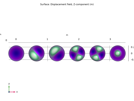
k10 = 2.4048
|
|||
|
k11 = 3.8317
|
|||
|
k11 = 3.8317
|
|||
|
k12 = 5.1356
|
|||
|
k12 = 5.1356
|
|||
|
k20 = 5.5201
|
|
1
|
|
2
|
|
3
|
Click Add.
|
|
4
|
Click
|
|
5
|
|
6
|
Click
|
|
1
|
|
2
|
|
1
|
|
2
|
|
1
|
|
2
|
|
3
|
|
1
|
|
2
|
|
3
|
|
4
|
|
5
|
|
1
|
In the Model Builder window, under Component 1 (comp1) right-click Materials and choose Blank Material.
|
|
2
|
|
1
|
In the Model Builder window, under Component 1 (comp1) > Membrane (mbrn) click Thickness and Offset 1.
|
|
2
|
|
3
|
|
1
|
|
2
|
|
3
|
|
1
|
|
3
|
|
4
|
|
1
|
|
1
|
|
3
|
|
4
|
|
1
|
|
2
|
|
3
|
|
4
|
Click
|
|
1
|
|
2
|
|
3
|
Select the Include geometric nonlinearity checkbox.
|
|
4
|
|
1
|
|
2
|
|
3
|
|
4
|
|
1
|
|
2
|
|
3
|
|
1
|
|
2
|
|
3
|
|
1
|
|
2
|
Go to the Add Study window.
|
|
3
|
Find the Studies subsection. In the Select Study tree, select Preset Studies for Selected Physics Interfaces > Eigenfrequency, Prestressed.
|
|
4
|
Click the Add Study button in the window toolbar.
|
|
5
|
|
1
|
|
3
|
|
4
|
|
5
|
|
1
|
|
1
|
|
2
|
|
3
|
Select the Modify model configuration for study step checkbox.
|
|
4
|
In the tree, select Component 1 (comp1) > Membrane (mbrn), Controls spatial frame > Linear Elastic Material 1 > Initial Stress and Strain 1.
|
|
5
|
Right-click and choose Disable.
|
|
1
|
|
2
|
|
3
|
Select the Modify model configuration for study step checkbox.
|
|
4
|
In the tree, select Component 1 (comp1) > Membrane (mbrn), Controls spatial frame > Linear Elastic Material 1 > Initial Stress and Strain 1.
|
|
5
|
Right-click and choose Disable.
|
|
6
|
|
1
|
|
2
|
|
3
|
|
4
|
|
1
|
|
2
|
|
3
|
|
1
|
|
2
|
|
1
|
In the Model Builder window, expand the Study 1 > Solver Configurations node, then click Study 1 > Step 1: Eigenfrequency.
|
|
2
|
|
3
|
Select the Modify model configuration for study step checkbox.
|
|
4
|
|
5
|
Click
|