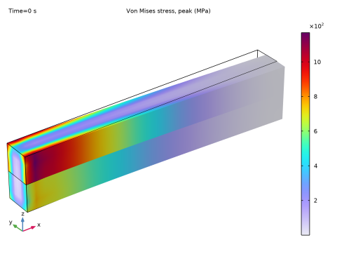
PDF

Heat Generation in a Vibrating Structure
Introduction
When a structure is subjected to vibrations of high frequency, a significant amount of heat can be generated within the structure because of mechanical losses in the material such as, for example, viscoelastic effects.
In this example, you model the slow rise of the temperature in a vibrating beam-like structure. You use a transient heat-transfer problem with source term which represents the heat generation due to mechanical losses. The simulation is based on a structural analysis performed in the frequency domain.
Model Definition
The beam consists of two layers made of aluminum and titanium, respectively, with the corresponding loss factors 0.001 and 0.005. One end of the beam is fixed, and the other one is subjected to periodic loading in the z direction, which is represented in the frequency domain as Fyexp(jωt), where j is the imaginary unit, and the angular frequency is
The excitation frequency 7760 Hz and the load magnitude Fy =  0.05 MPa are used in this example. The frequency is close to the first natural frequency of the structure.
The temperature rise is given by the heat-transfer equation
where k is the thermal conductivity, and the volumetric heat capacity ρCp is independent of the temperature in accordance with the Dulong-Petit law.
Note that T represents the temperature averaged over the time period 2π/ω. The heat source
presents the internal work of the nonelastic (for example, viscous) forces over the period. In the above expression, η is the loss factor, ε is the strain tensor, and is the elasticity tensor. The term is computed from a structural analysis performed in the frequency domain.
The initial state at time = 0 is stress-free, and the initial temperature is 293.15 K over the entire beam.
Use the following boundary conditions:
where h = 5 W/(m2·K) is the heat transfer coefficient and Text  = 293.15 K is the external temperature.
For the simulation, apply a periodic loading in the y direction of magnitude 0.05 MPa and frequency 7760 Hz at the free end of the beam for 2 seconds, keeping the fixed end and the structure environment at a constant temperature of 300 K during the process.
Results and Discussion
The stress solution computed in frequency domain is shown in Figure 1. It appears that the maximum stresses are located at the fixed end. As consequence more energy is dissipated at this location.
Figure 1: von Mises stress from the frequency domain solution.
Figure 2 displays the temperature distribution at the end of the simulated 2-second forced vibrations. As the figure shows, the maximum temperature rise in the beam is about 27.6 K.
Figure 2: Temperature increase in the beam after 2 seconds of forced vibrations.
The maximum temperature increase is plotted in Figure 3, it shows that the maximum temperature increases in the first time steps, then starts to stabilize around the end time.
Figure 3: Maximum temperature increase with time.
Application Library path: Structural_Mechanics_Module/Thermal-Structure_Interaction/vibrating_beam
Modeling Instructions
From the File menu, choose New.
New
In the New window, click  Model Wizard.
Model Wizard
1
In the Model Wizard window, click  3D.
2
In the Select Physics tree, select Heat Transfer > Heat Transfer in Solids (ht).
3
Click Add.
4
In the Select Physics tree, select Structural Mechanics > Solid Mechanics (solid).
5
Click Add.
6
Click  Study.
7
In the Select Study tree, select General Studies > Time Dependent.
8
Geometry 1
Block 1 (blk1)
1
In the Geometry toolbar, click  Block.
2
In the Settings window for Block, locate the Size and Shape section.
3
In the Width text field, type 0.01.
4
In the Depth text field, type 0.001.
5
In the Height text field, type 0.001.
Block 2 (blk2)
1
In the Geometry toolbar, click  Block.
2
In the Settings window for Block, locate the Size and Shape section.
3
In the Width text field, type 0.01.
4
In the Depth text field, type 0.001.
5
In the Height text field, type 0.001.
6
Locate the Position section. In the z text field, type 0.001.
7
In the Model Builder window, right-click Geometry 1 and choose Build All Objects.
Add Material
1
In the Materials toolbar, click  Add Material to open the Add Material window.
2
Go to the Add Material window.
3
In the tree, select Built-in > Aluminum.
4
Click the Add to Component button in the window toolbar.
5
In the tree, select Built-in > Titanium beta-21S.
6
Click the Add to Component button in the window toolbar.
7
In the Materials toolbar, click  Add Material to close the Add Material window.
Materials
Aluminum (mat1)
Select Domain 1 only.
Titanium beta-21S (mat2)
1
In the Model Builder window, click Titanium beta-21S (mat2).
2
Solid Mechanics (solid)
Fixed Constraint 1
1
In the Physics toolbar, click  Boundaries and choose Fixed Constraint.
2
Boundary Load 1
1
In the Physics toolbar, click  Boundaries and choose Boundary Load.
2
3
In the Settings window for Boundary Load, locate the Force section.
4
Specify the fA vector as
Linear Elastic Material 1
In the Model Builder window, click Linear Elastic Material 1.
Damping 1
1
In the Physics toolbar, click  Attributes and choose Damping.
2
3
In the Settings window for Damping, locate the Damping Settings section.
4
From the Damping type list, choose Isotropic loss factor.
5
From the ηs list, choose User defined. In the associated text field, type 0.001.
Linear Elastic Material 1
In the Model Builder window, click Linear Elastic Material 1.
Damping 2
1
In the Physics toolbar, click  Attributes and choose Damping.
2
3
In the Settings window for Damping, locate the Damping Settings section.
4
From the Damping type list, choose Isotropic loss factor.
5
From the ηs list, choose User defined. In the associated text field, type 0.005.
Heat Transfer in Solids (ht)
In the Model Builder window, under Component 1 (comp1) click Heat Transfer in Solids (ht).
Temperature 1
1
In the Physics toolbar, click  Boundaries and choose Temperature.
2
Heat Flux 1
1
In the Physics toolbar, click  Boundaries and choose Heat Flux.
2
In the Settings window for Heat Flux, locate the Heat Flux section.
3
From the Flux type list, choose Convective heat flux.
4
In the h text field, type 5.
5
Heat Source 1
1
In the Physics toolbar, click  Domains and choose Heat Source.
2
In the Settings window for Heat Source, locate the Domain Selection section.
3
From the Selection list, choose All domains.
4
Locate the Heat Source section. From the Q0 list, choose Total power dissipation density (solid).
This choice models the heat generated by the vibrations in the structure.
Definitions
Maximum 1 (maxop1)
1
In the Definitions toolbar, click  Nonlocal Couplings and choose Maximum.
Add a maximum operator to enable the calculation of maximum temperature after computation.
2
In the Settings window for Maximum, locate the Source Selection section.
3
From the Selection list, choose All domains.
Mesh 1
1
In the Model Builder window, under Component 1 (comp1) click Mesh 1.
2
In the Settings window for Mesh, locate the Physics-Controlled Mesh section.
3
From the Element size list, choose Extra fine.
Swept 1
1
In the Mesh toolbar, click  Swept.
2
In the Settings window for Swept, click  Build All.
Study 1
Step 1: Time Dependent
1
In the Model Builder window, under Study 1 click Step 1: Time Dependent.
2
In the Settings window for Time Dependent, locate the Study Settings section.
3
In the Output times text field, type range(0,0.05,2).
You need to set up the Solid Mechanics equation form to frequency-domain. The time dependent equations should be applied to the heat transfer physics only.
4
Locate the Physics and Variables Selection section. Select the Modify model configuration for study step checkbox.
5
In the tree, select Component 1 (comp1) > Solid Mechanics (solid).
6
From the Equation form list, choose Frequency domain.
7
In the Frequency text field, type 7760[Hz].
This frequency is close to the first natural frequency of the structure.
Before computing the solution, generate the default plots.
8
In the Model Builder window, right-click Study 1 and choose Get Initial Value for Step.
Results
Volume 1
1
In the Model Builder window, expand the Temperature (ht) node, then click Volume 1.
2
In the Settings window for Volume, locate the Expression section.
3
In the Expression text field, type T-293.15.
Study 1
Step 1: Time Dependent
1
In the Model Builder window, under Study 1 click Step 1: Time Dependent.
2
In the Settings window for Time Dependent, click to expand the Results While Solving section.
3
Select the Plot checkbox.
Solver Configurations
In the Model Builder window, expand the Study 1 > Solver Configurations node.
Solution 1 (sol1)
1
In the Model Builder window, expand the Study 1 > Solver Configurations > Solution 1 (sol1) node, then click Time-Dependent Solver 1.
2
In the Settings window for Time-Dependent Solver, click to expand the Time Stepping section.
3
From the Steps taken by solver list, choose Intermediate.
You need to enable complex values because they are used in the solid mechanics equations, which you have manually reconfigured for the frequency-domain analysis.
4
Click to expand the Advanced section. Select the Allow complex numbers checkbox.
5
In the Study toolbar, click  Compute.
Results
Temperature (ht)
1
In the Settings window for 3D Plot Group, locate the Color Legend section.
2
Select the Show maximum and minimum values checkbox.
3
In the Temperature (ht) toolbar, click  Plot.
The computed solution should closely resemble that shown in Figure 2.
Volume 1
1
In the Model Builder window, expand the Stress (solid) node, then click Volume 1.
2
In the Settings window for Volume, locate the Expression section.
3
From the Unit list, choose MPa.
4
In the Stress (solid) toolbar, click  Plot.
Temperature Increase
1
In the Home toolbar, click  Add Plot Group and choose 1D Plot Group.
2
In the Settings window for 1D Plot Group, type Temperature Increase in the Label text field.
Global 1
1
In the Temperature Increase toolbar, click  Global.
2
In the Settings window for Global, locate the y-Axis Data section.
3
4
Click to expand the Legends section. Clear the Show legends checkbox.