|
|
|
|
1.8e-3 s
|
|
|
1
|
|
2
|
|
3
|
Click Add.
|
|
4
|
|
5
|
Click Add.
|
|
6
|
|
7
|
Click Add.
|
|
8
|
|
9
|
Click Add.
|
|
10
|
In the Select Physics tree, select Mathematics > ODE and DAE Interfaces > Domain ODEs and DAEs (dode).
|
|
11
|
Click Add.
|
|
12
|
Click
|
|
13
|
|
14
|
Click
|
|
1
|
|
2
|
|
4
|
|
1
|
|
2
|
|
4
|
|
1
|
|
2
|
|
50 Ω
|
|||
|
3.132E-8 Ω·m
|
|||
|
4
|
|
1
|
|
2
|
|
4
|
|
1
|
|
2
|
|
3
|
|
4
|
Click
|
|
5
|
Browse to the model’s Application Libraries folder and double-click the file vacancy_electromigration_hydrostatic_stress.txt.
|
|
6
|
Locate the Interpolation and Extrapolation section. From the Interpolation list, choose Piecewise cubic.
|
|
7
|
Locate the Data Column Settings section. In the table, click to select the cell at row number 1 and column number 1.
|
|
8
|
|
10
|
|
11
|
|
1
|
|
2
|
|
3
|
|
4
|
Click
|
|
5
|
Browse to the model’s Application Libraries folder and double-click the file vacancy_electromigration_hydrostatic_stress_steady.txt.
|
|
6
|
Locate the Interpolation and Extrapolation section. From the Interpolation list, choose Piecewise cubic.
|
|
7
|
Locate the Data Column Settings section. In the table, click to select the cell at row number 1 and column number 1.
|
|
8
|
|
10
|
|
11
|
|
1
|
|
2
|
|
3
|
|
4
|
Click
|
|
5
|
Browse to the model’s Application Libraries folder and double-click the file vacancy_electromigration_anode_stress.txt.
|
|
6
|
Locate the Interpolation and Extrapolation section. From the Interpolation list, choose Piecewise cubic.
|
|
7
|
Locate the Data Column Settings section. In the table, click to select the cell at row number 1 and column number 1.
|
|
8
|
|
10
|
|
11
|
|
1
|
|
2
|
|
3
|
|
4
|
Click
|
|
5
|
Browse to the model’s Application Libraries folder and double-click the file vacancy_electromigration_cathode_stress.txt.
|
|
6
|
Locate the Interpolation and Extrapolation section. From the Interpolation list, choose Piecewise cubic.
|
|
7
|
Locate the Data Column Settings section. In the table, click to select the cell at row number 1 and column number 1.
|
|
8
|
|
10
|
|
11
|
|
1
|
|
2
|
|
3
|
|
4
|
Click
|
|
5
|
Browse to the model’s Application Libraries folder and double-click the file vacancy_electromigration_cathode_concentration.txt.
|
|
6
|
Locate the Data Column Settings section. In the table, click to select the cell at row number 1 and column number 1.
|
|
7
|
|
9
|
|
10
|
|
1
|
|
2
|
|
3
|
|
4
|
Click
|
|
5
|
Browse to the model’s Application Libraries folder and double-click the file vacancy_electromigration_anode_concentration.txt.
|
|
6
|
Locate the Data Column Settings section. In the table, click to select the cell at row number 1 and column number 1.
|
|
7
|
|
9
|
|
10
|
|
1
|
In the Model Builder window, under Global Definitions, Ctrl-click to select Hydrostatic Stress at t=70[s] (int1), Steady State Hydrostatic Stress (int2), Stress vs. Time, Anode (int3), Stress vs. Time, Cathode (int4), Concentration vs. Time, Cathode (int5), and Concentration vs. Time, Anode (int6).
|
|
2
|
Right-click and choose Group.
|
|
1
|
|
2
|
|
3
|
|
1
|
|
2
|
|
3
|
|
4
|
|
1
|
|
2
|
Go to the Add Material window.
|
|
3
|
|
4
|
Click the Add to Component button in the window toolbar.
|
|
5
|
|
1
|
|
2
|
|
3
|
|
1
|
In the Model Builder window, under Component 1 (comp1) > Heat Transfer in Solids (ht) click Initial Values 1.
|
|
2
|
|
3
|
|
1
|
|
3
|
|
4
|
|
1
|
In the Model Builder window, under Component 1 (comp1) right-click Definitions and choose Variables.
|
|
2
|
|
3
|
Click
|
|
4
|
Browse to the model’s Application Libraries folder and double-click the file vacancy_electromigration_variables.txt.
|
|
1
|
|
2
|
|
3
|
|
1
|
In the Model Builder window, under Component 1 (comp1) > Electric Currents (ec) click Current Conservation in Solids 1.
|
|
2
|
In the Settings window for Current Conservation in Solids, locate the Constitutive Relation Jc-E section.
|
|
3
|
|
4
|
|
5
|
|
6
|
|
1
|
|
3
|
|
1
|
|
3
|
|
4
|
|
5
|
|
1
|
|
2
|
|
3
|
|
4
|
|
5
|
|
1
|
|
2
|
|
3
|
|
1
|
|
2
|
|
3
|
|
1
|
|
3
|
|
4
|
|
1
|
|
2
|
|
3
|
|
4
|
|
1
|
|
2
|
|
3
|
|
4
|
|
1
|
|
2
|
|
3
|
|
1
|
|
2
|
|
3
|
|
4
|
|
5
|
In the Dependent variables (1) table, enter the following settings:
|
|
6
|
|
1
|
In the Model Builder window, under Component 1 (comp1) > Domain ODEs and DAEs (dode) click Distributed ODE 1.
|
|
2
|
|
3
|
|
1
|
|
2
|
|
3
|
|
4
|
|
5
|
Click to expand the Discretization section.
|
|
1
|
|
2
|
Click in the Graphics window and then press Ctrl+A to select all boundaries.
|
|
1
|
|
2
|
|
3
|
|
4
|
|
1
|
|
3
|
|
4
|
|
1
|
|
3
|
|
4
|
|
5
|
|
6
|
|
7
|
Select the Symmetric distribution checkbox.
|
|
8
|
Click
|
|
1
|
|
2
|
|
3
|
In the Output times text field, type 0 40 50 60 70 80 range(500,500,3500) 24000 25200 26000 range(40000,10000,190000) range(200000,100000,1400000).
|
|
4
|
|
1
|
|
2
|
|
3
|
|
4
|
|
1
|
|
2
|
|
3
|
|
4
|
|
5
|
|
1
|
|
2
|
|
3
|
|
4
|
|
5
|
|
6
|
|
7
|
|
8
|
|
9
|
Locate the Plot Settings section.
|
|
10
|
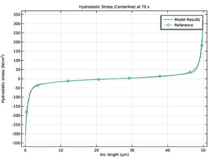
Select the y-axis label checkbox. In the associated text field, type Hydrostatic stress (N/cm<sup>2</sup>).
|
|
1
|
|
2
|
|
3
|
|
4
|
|
5
|
|
6
|
|
8
|
|
1
|
In the Model Builder window, right-click Hydrostatic Stress (Centerline) at 70 s and choose Line Graph.
|
|
2
|
|
3
|
|
4
|
|
5
|
Click to expand the Coloring and Style section. Find the Line style subsection. From the Line list, choose Dashed.
|
|
6
|
|
7
|
|
8
|
|
9
|
|
11
|
|
12
|
|
1
|
|
2
|
|
3
|
|
4
|
|
1
|
In the Model Builder window, expand the Hydrostatic Stress at Steady State (Centerline) node, then click Results for Validation.
|
|
2
|
|
3
|
|
4
|
|
1
|
|
2
|
|
3
|
|
4
|
|
5
|
|
1
|
|
2
|
|
3
|
|
4
|
|
1
|
|
2
|
|
3
|
|
4
|
Locate the Plot Settings section.
|
|
5
|
Select the y-axis label checkbox. In the associated text field, type Hydrostatic stress (N/cm<sup>2</sup>).
|
|
6
|
|
1
|
|
2
|
|
3
|
|
4
|
|
5
|
|
6
|
|
7
|
|
9
|
Select the Show legends checkbox.
|
|
10
|
|
1
|
|
2
|
|
3
|
|
4
|
Locate the Legends section. In the table, enter the following settings:
|
|
5
|
|
1
|
|
2
|
|
3
|
|
4
|
Locate the y-Axis Data section. In the table, enter the following settings:
|
|
5
|
Click to expand the Coloring and Style section. Find the Line style subsection. From the Line list, choose Dashed.
|
|
6
|
|
7
|
|
8
|
|
9
|
|
1
|
|
2
|
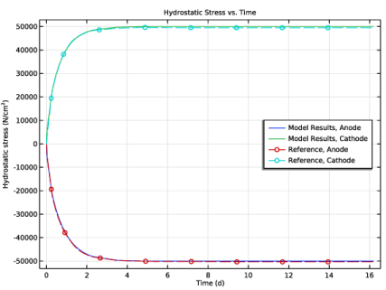
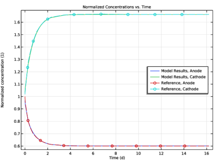
In the Settings window for 1D Plot Group, type Normalized Concentrations vs. Time in the Label text field.
|
|
3
|
Locate the Plot Settings section. In the y-axis label text field, type Normalized concentration (1).
|
|
1
|
In the Model Builder window, expand the Normalized Concentrations vs. Time node, then click Model Results Anode.
|
|
2
|
|
3
|
|
1
|
|
2
|
|
3
|
|
1
|
|
2
|
|
4
|