PDF

Instability of Two Contacting Arches
Introduction
This conceptual example shows how to calculate critical points in models with contact. The model consists of two contacting arches modeled with the Shell interface. During loading, the lower arch exhibits a snap-through behavior. The definition of the problem is based on a benchmark example from Ref. 1.
A similar example can be found in the Application Library: Block Pressing on Arch, where a block modeled with the Solid Mechanics interface pressing on an arch modeled with the Shell interface is analyzed.
Model Definition
The model geometry consists of an arch and a block as shown in Figure 1. Since the arches are modeled with the Shell interface, a 3D geometry is used. However, a 2D plane strain behavior is intended, and consequently symmetry conditions are applied to all edges in the y direction to suppress any out-of-plane deformation
.
Figure 1: Model geometry.
Only contact without friction is considered and the penalty contact method is used.
The ends of the upper arch are constrained against displacement in the x direction and subjected to vertical edge loads. The magnitude of the edge loads is controlled by the monotonically increasing deflection of the upper arch, which makes it possible to track the entire load path, even though the force does not increase monotonically. The ends of the lower arch are fixed.
Results and Discussion
Figure 2 depicts the deformed shape and the von Mises stress distribution at the last step of the simulation. The snap-through of the lower arch is clearly visible. Both arches are represented by a shell dataset that shows both their top and bottom surfaces.
Figure 2: Deformation and von Mises stress at the final step.
Three different load versus deflection curves are shown in Figure 3. The load is represented by a dimensionless load factor, and is plotted against either the mid deflections of the two arches or the average deflection of the ends of the upper arch. Several critical points can be observed. For example, looking at the lower arch, a first limit point is reached for a load factor equal to 107.5 and a deflection of 13 mm. At this point the lower arch becomes unstable and a snap-through occurs. When the deflection reaches 45 mm, the load factor has decreased to 45. At this point a second limit point is reached, and the model finds a new stable configuration. After this point the load factor increases with increasing deflection.
Several bifurcation points are also present, indicating the unstable nature of the problem and possible branching of the load path. A first point is, for example, visible already at a deflection of 1 mm, where there is a clear change in the slope of the load-deflection curve.
Figure 3: Load versus deflection curves.
The progressive deformation of the two arches, including the snap-through of the lower arch, is shown in Figure 4 for five values of the continuation parameter. In the figure, it also is clearly visible how the contact problem changes throughout the simulation. Figure 5 shows the contact pressure exerted by the upper arch on the lower arch during the postcritical stage.
Figure 4: Deformation of the model for five different parameter values.
Figure 5: Contact pressure acting on the lower arch.
Notes About the COMSOL Implementation
Modeling the postcritical behavior of a system is not possible by incrementally increasing the boundary load. The unstable behavior is even more pronounced when contact is present. To be able to find all limit points and to track the full load versus deflection curve, a displacement controlled load scheme is used by adding a Global Equation. Here, the magnitude of the edge loads is controlled through the monotonically increasing deflection of the upper arch. Alternatively, the vertical displacement could be prescribed on end points of the upper arch, but this is a less general technique that fails for some cases.
This problem is highly unstable and several branches of the equilibrium path are possible. To suppress these so that a stable solution is obtained, the mid-point of both arches is constrained against sideways displacement through a symmetry condition. By deactivating this constraint, it is possible to study the branching of the equilibrium path.
Reference
1. P. Wriggers, Computational Contact Mechanics, Springer-Verlag, 2006
Application Library path: Structural_Mechanics_Module/Verification_Examples/two_arches
Modeling Instructions
From the File menu, choose New.
New
In the New window, click  Model Wizard.
Model Wizard
1
In the Model Wizard window, click  3D.
2
In the Select Physics tree, select Structural Mechanics > Shell (shell).
3
Click Add.
4
Click  Study.
5
In the Select Study tree, select General Studies > Stationary.
6
Global Definitions
Parameters 1
1
In the Model Builder window, under Global Definitions click Parameters 1.
2
In the Settings window for Parameters, locate the Parameters section.
3
Click  Load from File.
4
Geometry 1
Work Plane 1 (wp1)
1
In the Geometry toolbar, click  Work Plane.
2
In the Settings window for Work Plane, locate the Plane Definition section.
3
From the Plane list, choose xz-plane.
4
Click  Go to Plane Geometry.
Work Plane 1 (wp1) > Circle 1 (c1)
1
In the Work Plane toolbar, click  Circle.
2
In the Settings window for Circle, locate the Object Type section.
3
From the Type list, choose Curve.
4
Locate the Size and Shape section. In the Radius text field, type Ri_upper.
5
In the Sector angle text field, type seg_upper.
6
Locate the Position section. In the yw text field, type Ri_upper.
7
Locate the Rotation Angle section. In the Rotation text field, type -90-seg_upper/2.
8
Click  Build Selected.
9
Click the  Zoom Extents button in the Graphics toolbar.
Work Plane 1 (wp1) > Circle 2 (c2)
1
In the Work Plane toolbar, click  Circle.
2
In the Settings window for Circle, locate the Object Type section.
3
From the Type list, choose Curve.
4
Locate the Size and Shape section. In the Radius text field, type Ri_lower.
5
In the Sector angle text field, type seg_lower.
6
Locate the Position section. In the yw text field, type -Ri_lower.
7
Locate the Rotation Angle section. In the Rotation text field, type 90-seg_lower/2.
8
Click  Build Selected.
Work Plane 1 (wp1) > Delete Entities 1 (del1)
1
In the Model Builder window, right-click Plane Geometry and choose Delete Entities.
2
On the object c1, select Boundaries 2 and 3 only.
3
On the object c2, select Boundaries 3 and 4 only.
Work Plane 1 (wp1) > Partition Edges 1 (pare1)
1
In the Work Plane toolbar, click  Booleans and Partitions and choose Partition Edges.
2
On the object del1(1), select Boundary 1 only.
Work Plane 1 (wp1)
1
In the Model Builder window, under Component 1 (comp1) > Geometry 1 click Work Plane 1 (wp1).
2
In the Settings window for Work Plane, locate the Unite Objects section.
3
Clear the Unite objects checkbox.
Extrude 1 (ext1)
1
In the Geometry toolbar, click  Extrude.
2
In the Settings window for Extrude, locate the Distances section.
3
4
Click  Build Selected.
Upper Arch
1
In the Geometry toolbar, click  Selections and choose Explicit Selection.
2
In the Settings window for Explicit Selection, type Upper Arch in the Label text field.
3
Locate the Entities to Select section. From the Geometric entity level list, choose Object.
4
Select the object ext1(2) only.
5
Locate the Color section. From the Color list, choose Color 4.
6
Click  Build Selected.
Lower Arch
1
Right-click Upper Arch and choose Duplicate.
2
In the Settings window for Explicit Selection, type Lower Arch in the Label text field.
3
Locate the Entities to Select section. In the list box, select ext1(2).
4
Select the object ext1(1) only.
5
Locate the Color section. From the Color list, choose Color 12.
Form Union (fin)
1
In the Model Builder window, under Component 1 (comp1) > Geometry 1 click Form Union (fin).
2
In the Settings window for Form Union/Assembly, locate the Form Union/Assembly section.
3
From the Action list, choose Form an assembly.
4
Click  Build Selected.
5
Click the  Zoom Extents button in the Graphics toolbar.
Materials
Material 1 (mat1)
1
In the Model Builder window, under Component 1 (comp1) right-click Materials and choose Blank Material.
2
In the Settings window for Material, locate the Geometric Entity Selection section.
3
From the Selection list, choose Lower Arch.
4
Locate the Material Contents section. In the table, enter the following settings:
Material 2 (mat2)
1
Right-click Materials and choose Blank Material.
2
In the Settings window for Material, locate the Geometric Entity Selection section.
3
From the Selection list, choose Upper Arch.
4
Locate the Material Contents section. In the table, enter the following settings:
Definitions
Average 1 (aveop1)
1
In the Definitions toolbar, click  Nonlocal Couplings and choose Average.
2
In the Settings window for Average, locate the Source Selection section.
3
From the Geometric entity level list, choose Point.
4
Average 2 (aveop2)
1
Right-click Average 1 (aveop1) and choose Duplicate.
2
In the Settings window for Average, locate the Source Selection section.
3
Click  Clear Selection.
4
Average 3 (aveop3)
1
Right-click Average 2 (aveop2) and choose Duplicate.
2
In the Settings window for Average, locate the Source Selection section.
3
Click  Clear Selection.
4
Variables 1
1
In the Model Builder window, right-click Definitions and choose Variables.
2
In the Settings window for Variables, locate the Variables section.
3
Contact Pair 1 (p1)
1
In the Definitions toolbar, click  Pairs and choose Contact Pair.
2
In the Settings window for Pair, locate the Source Boundaries section.
3
From the Selection list, choose Upper Arch.
4
Locate the Destination Boundaries section. From the Selection list, choose Lower Arch.
Shell (shell)
Thickness and Offset 1
1
In the Model Builder window, under Component 1 (comp1) > Shell (shell) click Thickness and Offset 1.
2
In the Settings window for Thickness and Offset, locate the Thickness and Offset section.
3
In the d0 text field, type d.
4
From the Position list, choose Top surface on boundary.
Symmetry 1
1
In the Physics toolbar, click  Edges and choose Symmetry.
2
Prescribed Displacement/Rotation 1
1
In the Physics toolbar, click  Edges and choose Prescribed Displacement/Rotation.
2
3
In the Settings window for Prescribed Displacement/Rotation, locate the Prescribed Displacement section.
4
From the Displacement in x direction list, choose Prescribed.
5
From the Displacement in y direction list, choose Prescribed.
Fixed Constraint 1
1
In the Physics toolbar, click  Edges and choose Fixed Constraint.
2
Several possible branches are possible during the snap-through. Adding a constraint to each arch enforces a symmetric and stable solution.
Symmetry 2
1
In the Physics toolbar, click  Edges and choose Symmetry.
2
Edge Load 1
1
In the Physics toolbar, click  Edges and choose Edge Load.
2
3
In the Settings window for Edge Load, locate the Force section.
4
Specify the fL vector as
The dependent variable load will be created in the next step using a global equation.
5
Click the  Show More Options button in the Model Builder toolbar.
6
In the Show More Options dialog, in the tree, select the checkbox for the node Physics > Equation Contributions.
7
Global Equations 1 (ODE1)
1
In the Physics toolbar, click  Global and choose Global Equations.
2
In the Settings window for Global Equations, locate the Global Equations section.
3
4
Locate the Units section. Click  Select Source Term Quantity.
5
In the Physical Quantity dialog, type displacement in the text field.
6
In the tree, select General > Displacement (m).
7
Mesh 1
Mapped 1
1
In the Mesh toolbar, click  More Generators and choose Mapped.
2
In the Settings window for Mapped, locate the Boundary Selection section.
3
From the Selection list, choose All boundaries.
Distribution 1
1
Right-click Mapped 1 and choose Distribution.
2
3
In the Settings window for Distribution, locate the Distribution section.
4
In the Number of elements text field, type n_elem_lower.
Distribution 2
1
In the Model Builder window, right-click Mapped 1 and choose Distribution.
2
3
In the Settings window for Distribution, locate the Distribution section.
4
In the Number of elements text field, type n_elem_upper.
5
In the Model Builder window, right-click Mesh 1 and choose Build All.
6
Click the  Zoom Extents button in the Graphics toolbar.
Study 1
Step 1: Stationary
1
In the Model Builder window, under Study 1 click Step 1: Stationary.
2
In the Settings window for Stationary, click to expand the Study Extensions section.
3
Select the Auxiliary sweep checkbox.
4
5
6
7
Locate the Study Settings section. From the Tolerance list, choose User controlled.
8
In the Relative tolerance text field, type 0.0005.
Solution 1 (sol1)
1
In the Study toolbar, click  Show Default Solver.
2
In the Model Builder window, expand the Solution 1 (sol1) node.
3
In the Model Builder window, expand the Study 1 > Solver Configurations > Solution 1 (sol1) > Stationary Solver 1 node, then click Parametric 1.
4
In the Settings window for Parametric, click to expand the Continuation section.
5
Select the Tuning of step size checkbox.
6
In the Minimum step size text field, type 1e-6.
7
Right-click Study 1 > Solver Configurations > Solution 1 (sol1) > Stationary Solver 1 > Parametric 1 and choose Stop Condition.
8
In the Settings window for Stop Condition, locate the Stop Expressions section.
9
10
11
Locate the Output at Stop section. From the Add solution list, choose Step before stop.
12
In the Model Builder window, under Study 1 > Solver Configurations > Solution 1 (sol1) > Stationary Solver 1 click Fully Coupled 1.
13
In the Settings window for Fully Coupled, click to expand the Method and Termination section.
14
From the Nonlinear method list, choose Constant (Newton).
15
In the Study toolbar, click  Compute.
Results
Preferred Units 1
1
In the Results toolbar, click  Configurations and choose Preferred Units.
2
In the Settings window for Preferred Units, locate the Units section.
3
Click  Add Physical Quantity.
4
In the Physical Quantity dialog, select Solid Mechanics > Stress tensor (N/m^2) in the tree.
5
6
In the Settings window for Preferred Units, locate the Units section.
7
8
Select the Apply conversions to expressions with the same dimensions checkbox.
9
Click  Apply.
Stress (shell)
1
In the Model Builder window, under Results click Stress (shell).
2
In the Stress (shell) toolbar, click  Plot.
3
Click the  Show Grid button in the Graphics toolbar.
4
Click the  Zoom Extents button in the Graphics toolbar.
Result Templates
1
In the Results toolbar, click  Result Templates to open the Result Templates window.
2
Go to the Result Templates window.
3
In the tree, select Study 1/Solution 1 (sol1) > Shell > Contact Forces (shell).
4
Click the Add Result Template button in the window toolbar.
5
In the Results toolbar, click  Result Templates to close the Result Templates window.
Results
Contact Forces (shell)
1
In the Settings window for 3D Plot Group, locate the Data section.
2
From the Parameter value (para) list, choose 0.6.
Contact 1, Pressure
1
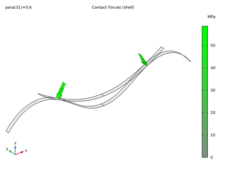
In the Model Builder window, expand the Contact Forces (shell) node, then click Contact 1, Pressure.
2
In the Settings window for Arrow Surface, locate the Coloring and Style section.
3
Select the Scale factor checkbox. In the associated text field, type 2e-4.
Gray Surfaces
In the Model Builder window, click Gray Surfaces.
Animation 1
1
In the Contact Forces (shell) toolbar, click  Animation and choose Player.
2
In the Settings window for Animation, locate the Frames section.
3
From the Frame selection list, choose All.
4
Click the  Play button in the Graphics toolbar.
Load vs. Deflection
1
In the Results toolbar, click  1D Plot Group.
2
In the Settings window for 1D Plot Group, type Load vs. Deflection in the Label text field.
Global 1
1
Right-click Load vs. Deflection and choose Global.
2
In the Settings window for Global, locate the y-Axis Data section.
3
4
Locate the x-Axis Data section. From the Parameter list, choose Expression.
5
In the Expression text field, type load.
6
Click to expand the Coloring and Style section. Find the Line markers subsection. From the Marker list, choose Cycle.
7
From the Positioning list, choose Interpolated.
Load vs. Deflection
1
In the Model Builder window, click Load vs. Deflection.
2
In the Settings window for 1D Plot Group, locate the Plot Settings section.
3
Select the Flip the x- and y-axes checkbox.
4
Locate the Legend section. From the Position list, choose Upper left.
5
Locate the Plot Settings section.
6
Select the x-axis label checkbox. In the associated text field, type Deflection (mm).
7
In the Load vs. Deflection toolbar, click  Plot.
Deformation
1
In the Results toolbar, click  1D Plot Group.
2
In the Settings window for 1D Plot Group, type Deformation in the Label text field.
3
Locate the Data section. From the Parameter selection (para) list, choose Manual.
4
In the Parameter indices (1-46) text field, type range(1,10,41).
5
Click to expand the Title section. From the Title type list, choose None.
Line Graph 1
1
Right-click Deformation and choose Line Graph.
2
3
In the Settings window for Line Graph, locate the y-Axis Data section.
4
In the Expression text field, type z.
5
Locate the x-Axis Data section. From the Parameter list, choose Expression.
6
In the Expression text field, type x.
7
Click to expand the Coloring and Style section. From the Width list, choose 2.
Line Graph 2
1
Right-click Line Graph 1 and choose Duplicate.
2
In the Settings window for Line Graph, locate the Selection section.
3
Click  Clear Selection.
4
5
Locate the Coloring and Style section. Find the Line style subsection. From the Line list, choose Dashed.
6
From the Color list, choose Cycle (reset).
Line Graph 1
1
In the Model Builder window, click Line Graph 1.
2
In the Settings window for Line Graph, click to expand the Legends section.
3
Select the Show legends checkbox.
4
Find the Prefix and suffix subsection. In the Prefix text field, type para = .
5
In the Deformation toolbar, click  Plot.