|
|
|
|
•
|
|
•
|
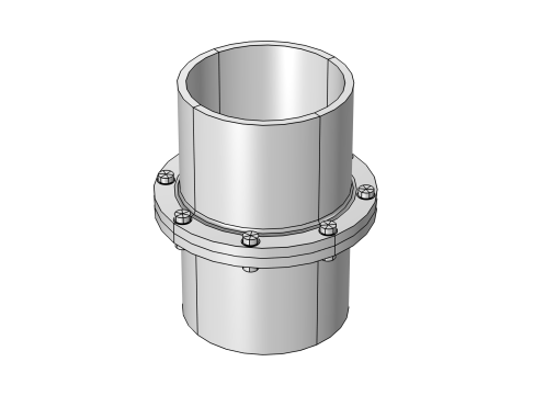
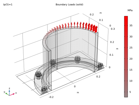
A constant axial force of 500 kN
|
|
1
|
|
2
|
|
3
|
Click Add.
|
|
4
|
Click
|
|
5
|
|
6
|
Click
|
|
1
|
|
2
|
|
3
|
Click
|
|
4
|
Browse to the model’s Application Libraries folder and double-click the file tube_connection_parameters.txt.
|
|
1
|
|
2
|
Browse to the model’s Application Libraries folder and double-click the file tube_connection_geom_sequence.mph.
|
|
1
|
|
2
|
|
3
|
|
4
|
|
5
|
|
6
|
Click
|
|
7
|
|
1
|
In the Model Builder window, expand the Component 1 (comp1) > Definitions node, then click Contact Pair 1 (ap1).
|
|
2
|
|
3
|
|
1
|
|
2
|
|
3
|
Click
|
|
4
|
|
5
|
Click OK.
|
|
6
|
|
1
|
|
2
|
|
3
|
Click the
|
|
1
|
|
2
|
|
3
|
Select the Manual control of selections and pair type checkbox.
|
|
4
|
|
1
|
In the Model Builder window, under Component 1 (comp1) > Definitions click Boundary System 1 (sys1).
|
|
2
|
|
3
|
|
1
|
|
2
|
|
3
|
|
4
|
|
5
|
|
6
|
|
1
|
|
2
|
|
3
|
|
4
|
|
5
|
In the Add dialog, in the Selections to add list, choose Bolts Symmetry and Symmetry Boundaries (xz-plane).
|
|
6
|
Click OK.
|
|
7
|
|
1
|
|
2
|
|
3
|
|
5
|
Select the Group by continuous tangent checkbox.
|
|
1
|
|
2
|
|
3
|
|
5
|
Select the Group by continuous tangent checkbox.
|
|
1
|
|
2
|
|
3
|
|
5
|
Select the Group by continuous tangent checkbox.
|
|
1
|
|
2
|
|
3
|
|
5
|
Select the Group by continuous tangent checkbox.
|
|
1
|
|
2
|
|
3
|
|
5
|
Select the Group by continuous tangent checkbox.
|
|
1
|
|
2
|
Go to the Add Material window.
|
|
3
|
|
4
|
Click the Add to Component button in the window toolbar.
|
|
5
|
|
1
|
|
2
|
|
4
|
|
5
|
|
1
|
|
2
|
In the Settings window for Boundary Load, type Bending Moment and Axial Force in the Label text field.
|
|
4
|
|
5
|
Specify the F vector as
|
|
6
|
Specify the M vector as
|
|
7
|
|
8
|
|
1
|
|
2
|
|
3
|
|
1
|
|
2
|
|
3
|
|
1
|
|
2
|
|
3
|
|
1
|
|
2
|
|
3
|
|
1
|
|
2
|
|
3
|
|
1
|
|
2
|
|
3
|
|
1
|
|
2
|
|
3
|
Click
|
|
4
|
|
5
|
Click OK.
|
|
6
|
|
7
|
From the list, choose Augmented Lagrangian.
|
|
8
|
|
1
|
|
2
|
|
3
|
|
1
|
|
2
|
|
3
|
|
1
|
|
2
|
|
3
|
|
1
|
|
3
|
|
4
|
|
1
|
|
3
|
In the Settings window for Stress Linearization, locate the Second Axis Orientation Reference Point section.
|
|
4
|
Click to select the
|
|
6
|
Repeat the previous steps to add Stress Linearization node for the edges 33, 36, 107, 110 and 115.
|
|
1
|
|
2
|
|
4
|
|
5
|
|
6
|
Select the Symmetry plane checkbox.
|
|
7
|
|
1
|
|
2
|
|
3
|
|
4
|
|
5
|
Click to expand the Source Faces section. Select Boundaries 59, 63, 67, 145, 149, and 153 only.
|
|
1
|
|
2
|
|
3
|
|
4
|
Click
|
|
1
|
|
2
|
|
3
|
|
4
|
|
1
|
|
2
|
|
3
|
|
1
|
|
2
|
|
3
|
|
4
|
Click
|
|
1
|
|
2
|
|
1
|
|
1
|
|
3
|
|
4
|
|
5
|
Click
|
|
1
|
|
2
|
|
3
|
|
1
|
|
2
|
|
3
|
|
4
|
Click
|
|
1
|
|
1
|
|
2
|
|
3
|
|
4
|
Click
|
|
1
|
|
2
|
|
1
|
|
1
|
|
3
|
|
4
|
|
5
|
Click
|
|
1
|
|
2
|
|
3
|
|
4
|
Locate the Physics and Variables Selection section. Select the Modify model configuration for study step checkbox.
|
|
5
|
In the tree, select Component 1 (comp1) > Solid Mechanics (solid), Controls spatial frame > Pressure.
|
|
6
|
Click
|
|
7
|
In the tree, select Component 1 (comp1) > Solid Mechanics (solid), Controls spatial frame > Bending Moment and Axial Force.
|
|
8
|
Click
|
|
1
|
|
2
|
|
3
|
Select the Auxiliary sweep checkbox.
|
|
4
|
Click
|
|
1
|
|
2
|
|
3
|
In the Model Builder window, expand the Study 1 > Solver Configurations > Solution 1 (sol1) > Dependent Variables 1 node, then click Displacement Field (comp1.u).
|
|
4
|
|
5
|
|
6
|
In the Model Builder window, expand the Study 1 > Solver Configurations > Solution 1 (sol1) > Dependent Variables 2 node, then click Displacement Field (comp1.u).
|
|
7
|
|
8
|
|
9
|
|
1
|
|
2
|
|
1
|
|
2
|
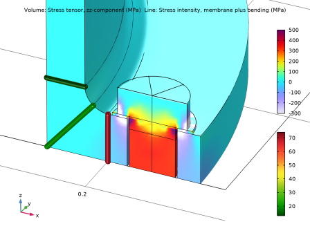
In the Settings window for Volume, click Replace Expression in the upper-right corner of the Expression section. From the menu, choose Component 1 (comp1) > Solid Mechanics > Stress > Stress tensor (spatial frame) - N/m² > solid.sGpzz - Stress tensor, zz-component.
|
|
3
|
|
4
|
|
5
|
|
1
|
|
2
|
|
3
|
|
1
|
|
2
|
|
3
|
Click
|
|
4
|
|
5
|
|
6
|
Click OK.
|
|
7
|
|
9
|
Select the Apply conversions to expressions with the same dimensions checkbox.
|
|
10
|
Click
|
|
1
|
|
2
|
|
1
|
|
2
|
|
3
|
|
4
|
Locate the Legends section. Find the Include in automatic mode subsection. Clear the Solution checkbox.
|
|
5
|
Select the Label checkbox.
|
|
6
|
Clear the Point checkbox.
|
|
1
|
|
2
|
|
3
|
|
4
|
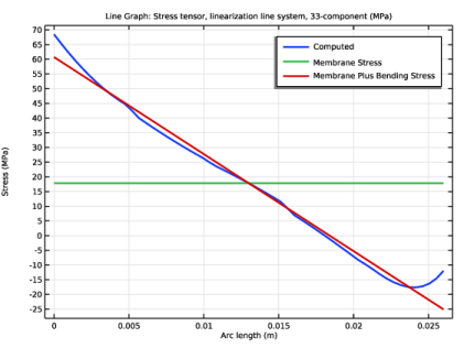
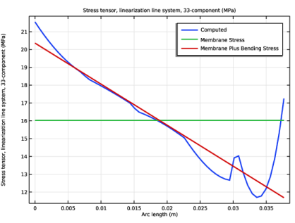
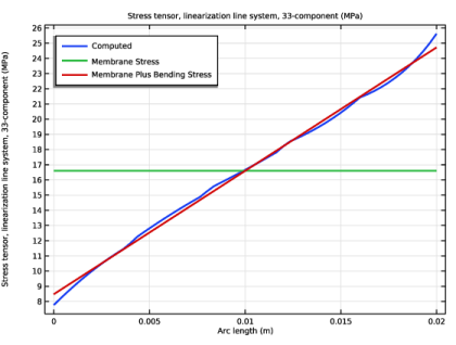
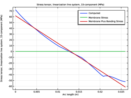
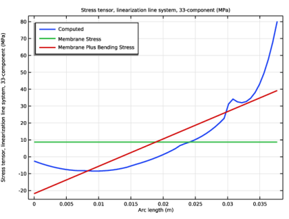
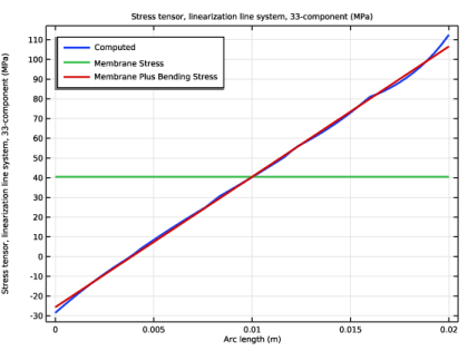
In the Title text area, type Line Graph: Stress tensor, linearization line system, 33-component (MPa).
|
|
5
|
|
6
|
|
7
|
Click to expand the Style Configuration section. From the Configuration list, choose Graph Plot Style 1.
|
|
8
|
|
2
|
Go to the Find and Replace window.
|
|
3
|
|
4
|
|
5
|
|
6
|
Click OK.
|
|
7
|
Go to the Find and Replace window.
|
|
8
|
|
9
|
|
10
|
Select the Case sensitive checkbox.
|
|
11
|
Click OK.
|
|
12
|
Go to the Find and Replace window.
|
|
13
|
|
14
|
|
15
|
Click
|
|
16
|
|
1
|
|
2
|
|
1
|
|
2
|
Go to the Result Templates window.
|
|
3
|
In the tree, select Study 1/Solution 1 (sol1) > Solid Mechanics > Section Forces (secf1) and Study 1/Solution 1 (sol1) > Solid Mechanics > Section Moments (secf1).
|
|
4
|
Click the Add Result Template button in the window toolbar.
|
|
5
|
|
1
|
In the Model Builder window, expand the Results > Section Moments (secf1) node, then click Annotation 1.
|
|
2
|
|
3
|
|
4
|
|
1
|
|
2
|
|
3
|
Clear the Plot dataset edges checkbox.
|
|
4
|
|
5
|
|
1
|
|
2
|
|
3
|
|
4
|
|
5
|
|
6
|
|
1
|
|
2
|
|
3
|
|
1
|
|
2
|
|
3
|
|
4
|
Clear the Color checkbox.
|
|
5
|
Clear the Color and data range checkbox.
|
|
6
|
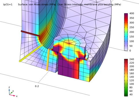
Click Replace Expression in the upper-right corner of the Expression section. From the menu, choose Component 1 (comp1) > Solid Mechanics > Stress linearization > solid.SImb - Stress intensity, membrane plus bending - N/m².
|
|
7
|
|
8
|
|
9
|
|
1
|
|
2
|
|
3
|
|
4
|
|
5
|
|
6
|
Select the Wireframe checkbox.
|
|
7
|
|
8
|
Clear the Color checkbox.
|
|
9
|
Clear the Color and data range checkbox.
|
|
1
|
|
2
|
|
1
|
|
2
|
|
1
|
|
2
|
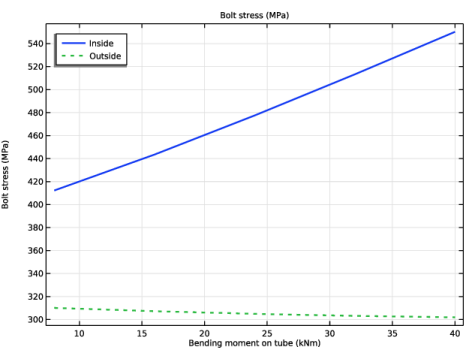
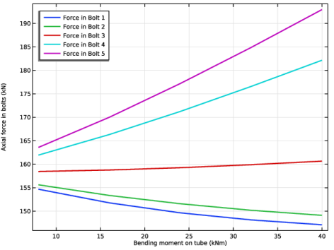
In the Settings window for Global, click Replace Expression in the upper-right corner of the y-Axis Data section. From the menu, choose Component 1 (comp1) > Solid Mechanics > Bolts > Bolt_1 > solid.pblt1.sblt1.F_bolt - Bolt force - N.
|
|
3
|
Locate the y-Axis Data section. In the table, enter the following settings:
|
|
4
|
|
5
|
|
6
|
|
7
|
|
1
|
|
2
|
|
3
|
|
4
|
|
1
|
|
2
|
|
3
|
Select the Show legends checkbox.
|
|
4
|
Click to collapse the Coloring and Style section.
|
|
1
|
|
2
|
|
3
|
|
4
|
|
1
|
|
2
|
|
1
|
|
3
|
In the Settings window for Point Graph, click Replace Expression in the upper-right corner of the y-Axis Data section. From the menu, choose Component 1 (comp1) > Solid Mechanics > Stress > Stress tensor (spatial frame) - N/m² > solid.sGpzz - Stress tensor, zz-component.
|
|
4
|
Locate the y-Axis Data section.
|
|
5
|
|
6
|
|
7
|
|
8
|
|
9
|
Click to expand the Coloring and Style section. Find the Line style subsection. From the Line list, choose Cycle.
|
|
10
|
|
11
|
|
12
|
|
1
|
|
2
|
|
3
|
|
4
|
|
1
|
|
2
|
|
3
|
|
1
|
|
2
|
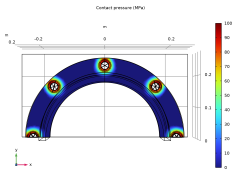
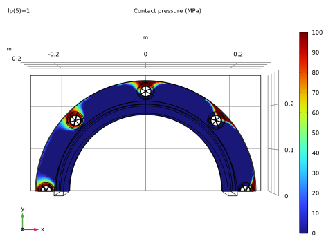
In the Settings window for Surface, click Replace Expression in the upper-right corner of the Expression section. From the menu, choose Component 1 (comp1) > Solid Mechanics > Contact > Contact 1 > solid.dcnt1.Tn - Contact pressure - N/m².
|
|
3
|
|
4
|
|
5
|
|
6
|
|
7
|
|
1
|
|
2
|
|
3
|
|
4
|
|
1
|
|
2
|
Go to the Result Templates window.
|
|
3
|
In the tree, select Study 1/Solution 1 (sol1) > Solid Mechanics > Applied Loads (solid) > Boundary Loads (solid).
|
|
4
|
Click the Add Result Template button in the window toolbar.
|
|
5
|
|
1
|
|
2
|