PDF

Thermally Loaded Beam
Introduction
In the following tutorial, you build and solve a 3D beam model using the 3D Beam interface. This example shows how to model a thermally induced deformation of a beam. Temperature gradients are applied between the top and bottom surfaces as well as between the left and right surfaces of the beam. The deformation is compared to the value given by a theoretical solution given in Ref. 1.
Model Definition
GEOMETRY
The geometry consists of one beam. The beam cross-section area is A and the area moment of inertia I. The beam is L long, and the Young’s modulus is E.
Beam length = 3 m.
The beam has a square cross section with a side length of 0.04 m giving an area of 1.6·103 m2 and an area moment of inertia of 0.044/12 m4.
Material
Young’s modulus 210 GPa.
Coefficient of thermal expansion α = 11·106/°C.
Constraints
Thermal Load
Figure 1 shows the surface temperature at each corner of the cross section. The temperature varies linearly between each corner. The deformation caused by this temperature distribution is modeled by specifying the temperature differences across the beam in the local y and z directions.
Figure 1: Geometric properties and thermal loads at corners.
Results and Discussion
Based on Ref. 1, you can compare the maximum deformation in the global z direction with analytical values for a simply supported 2D beam with a temperature difference between the top and the bottom surface. The maximum deformation, according to Ref. 1 is:
where t is the depth of the beam, 0.04 m, T2 is the temperature at the top and T1 at the bottom.
The following table shows a comparison of the maximum global z-displacement, calculated with COMSOL Multiphysics, with the theoretical solution.
Figure 2 shows the global z-displacement along the beam.
Figure 2: z-displacement along the beam.
The analytical values for the maximum total transverse displacement can be calculated by:
where v is the maximum deformation in the global y direction which is calculated in the same way as w.
A comparison of the maximum transverse displacement calculated with COMSOL Multiphysics and the analytical value is shown in the table below.
Figure 3 shows the total displacement, the total transverse displacement and the axial displacement along the beam.
Figure 3: Camber along the beam.
Reference
1. W. Young, Roark’s Formulas for Stress & Strain, McGraw Hill, 1989.
Application Library path: Structural_Mechanics_Module/Verification_Examples/thermally_loaded_beam
Modeling Instructions
From the File menu, choose New.
New
In the New window, click  Model Wizard.
Model Wizard
1
In the Model Wizard window, click  3D.
2
In the Select Physics tree, select Structural Mechanics > Beam (beam).
3
Click Add.
4
Click  Study.
5
In the Select Study tree, select General Studies > Stationary.
6
Global Definitions
Parameters 1
1
In the Model Builder window, under Global Definitions click Parameters 1.
2
In the Settings window for Parameters, locate the Parameters section.
3
Geometry 1
Polygon 1 (pol1)
1
In the Geometry toolbar, click  More Primitives and choose Polygon.
2
In the Settings window for Polygon, locate the Coordinates section.
3
Materials
Material 1 (mat1)
1
In the Model Builder window, under Component 1 (comp1) right-click Materials and choose Blank Material.
2
In the Settings window for Material, click to expand the Material Properties section.
3
In the Material properties tree, select Basic Properties > Coefficient of Thermal Expansion.
4
Click  Add to Material.
5
Locate the Material Contents section. In the table, enter the following settings:
Beam (beam)
Cross-Section Data 1
1
In the Model Builder window, under Component 1 (comp1) > Beam (beam) click Cross-Section Data 1.
2
In the Settings window for Cross-Section Data, locate the Cross-Section Definition section.
3
From the Section type list, choose Rectangle.
4
In the hy text field, type a.
5
In the hz text field, type a.
Section Orientation 1
1
In the Model Builder window, click Section Orientation 1.
2
In the Settings window for Section Orientation, locate the Section Orientation section.
3
From the Orientation method list, choose Orientation vector.
4
Specify the V vector as
Prescribed Displacement/Rotation 1
1
In the Physics toolbar, click  Points and choose Prescribed Displacement/Rotation.
2
3
In the Settings window for Prescribed Displacement/Rotation, locate the Prescribed Displacement section.
4
From the Displacement in x direction list, choose Prescribed.
5
From the Displacement in y direction list, choose Prescribed.
6
From the Displacement in z direction list, choose Prescribed.
7
Locate the Prescribed Rotation section. From the list, choose Rotation.
8
Select the Free rotation around y direction checkbox.
9
Select the Free rotation around z direction checkbox.
Prescribed Displacement/Rotation 2
1
In the Physics toolbar, click  Points and choose Prescribed Displacement/Rotation.
2
3
In the Settings window for Prescribed Displacement/Rotation, locate the Prescribed Displacement section.
4
From the Displacement in y direction list, choose Prescribed.
5
From the Displacement in z direction list, choose Prescribed.
Linear Elastic Material 1
In the Model Builder window, click Linear Elastic Material 1.
Thermal Expansion 1
1
In the Physics toolbar, click  Attributes and choose Thermal Expansion.
2
In the Settings window for Thermal Expansion, locate the Model Input section.
3
Click  Go to Source for Volume reference temperature.
Global Definitions
Default Model Inputs
1
In the Model Builder window, under Global Definitions click Default Model Inputs.
2
In the Settings window for Default Model Inputs, locate the Browse Model Inputs section.
3
Find the Expression for remaining selection subsection. In the Volume reference temperature text field, type 0.
Beam (beam)
Thermal Expansion 1
1
In the Model Builder window, under Component 1 (comp1) > Beam (beam) > Linear Elastic Material 1 click Thermal Expansion 1.
2
In the Settings window for Thermal Expansion, locate the Model Input section.
3
From the T list, choose User defined. In the associated text field, type 200.
4
Locate the Thermal Bending section. In the Tgy text field, type Tg.
5
In the Tgz text field, type -Tg.
Study 1
In the Study toolbar, click  Compute.
Set default units for result presentation.
Results
Preferred Units 1
1
In the Results toolbar, click  Configurations and choose Preferred Units.
2
In the Settings window for Preferred Units, locate the Units section.
3
Click  Add Physical Quantity.
4
In the Physical Quantity dialog, select General > Displacement (m) in the tree.
5
6
In the Settings window for Preferred Units, locate the Units section.
7
8
Select the Apply conversions to expressions with the same dimensions checkbox.
9
Click  Apply.
Displacement, 3D
1
In the Model Builder window, under Results click Stress, 3D (beam).
2
In the Settings window for 3D Plot Group, type Displacement, 3D in the Label text field.
Surface 1
1
In the Model Builder window, expand the Displacement, 3D node, then click Surface 1.
2
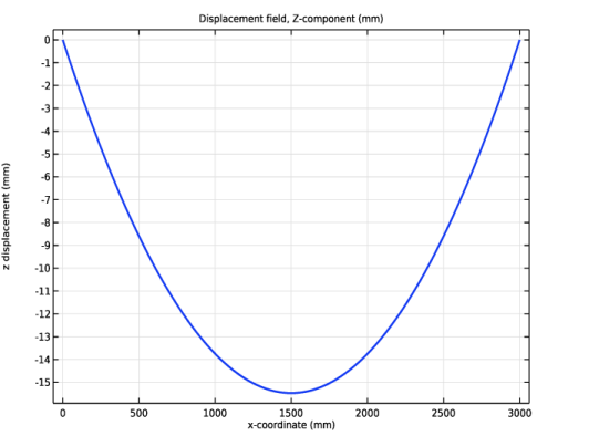
In the Settings window for Surface, click Replace Expression in the upper-right corner of the Expression section. From the menu, choose Component 1 (comp1) > Beam > Displacement > beam.disp - Displacement magnitude - m.
3
Locate the Coloring and Style section. From the Color table list, choose SpectrumLight.
4
In the Displacement, 3D toolbar, click  Plot.
Transverse Displacement
1
In the Results toolbar, click  1D Plot Group.
2
In the Settings window for 1D Plot Group, type Transverse Displacement in the Label text field.
3
Locate the Plot Settings section.
4
Select the y-axis label checkbox. In the associated text field, type z displacement (mm).
Transverse displacement (z direction)
1
Right-click Transverse Displacement and choose Line Graph.
2
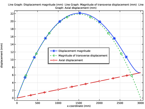
In the Settings window for Line Graph, type Transverse displacement (z direction) in the Label text field.
3
Click in the Graphics window and then press Ctrl+A to select both edges.
4
Locate the y-Axis Data section. In the Expression text field, type w.
5
Locate the x-Axis Data section. From the Parameter list, choose Expression.
6
In the Expression text field, type x.
7
Click to expand the Coloring and Style section. From the Width list, choose 2.
8
In the Transverse Displacement toolbar, click  Plot.
Displacement
1
In the Results toolbar, click  1D Plot Group.
2
In the Settings window for 1D Plot Group, type Displacement in the Label text field.
3
Locate the Plot Settings section.
4
Select the y-axis label checkbox. In the associated text field, type displacement (mm).
5
Locate the Legend section. From the Position list, choose Center.
Displacement magnitude
1
Right-click Displacement and choose Line Graph.
2
In the Settings window for Line Graph, type Displacement magnitude in the Label text field.
3
Click in the Graphics window and then press Ctrl+A to select both edges.
4
Locate the y-Axis Data section. Select the Description checkbox.
5
Locate the x-Axis Data section. From the Parameter list, choose Expression.
6
In the Expression text field, type x.
7
Locate the Coloring and Style section. Find the Line style subsection. From the Line list, choose Cycle.
8
Find the Line markers subsection. From the Marker list, choose Cycle.
9
From the Positioning list, choose Interpolated.
10
From the Width list, choose 2.
11
Click to expand the Legends section. Find the Include subsection. Select the Description checkbox.
12
Clear the Solution checkbox.
13
Select the Show legends checkbox.
Magnitude of transverse displacement
1
Right-click Displacement magnitude and choose Duplicate.
2
In the Settings window for Line Graph, type Magnitude of transverse displacement in the Label text field.
3
Locate the Selection section. Click to select the  Activate Selection toggle button.
4
Locate the y-Axis Data section. In the Expression text field, type sqrt(v^2+w^2).
5
In the Description text field, type Magnitude of transverse displacement.
Axial displacement
1
Right-click Magnitude of transverse displacement and choose Duplicate.
2
In the Settings window for Line Graph, type Axial displacement in the Label text field.
3
Locate the y-Axis Data section. In the Expression text field, type u.
4
In the Description text field, type Axial displacement.
5
In the Displacement toolbar, click  Plot.